How do I create a boxplot from my data?

Worked-out example:

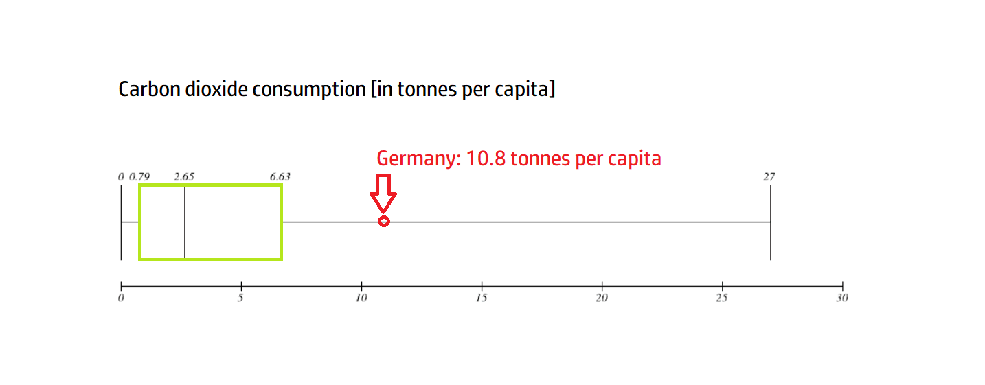
Carbon dioxide consumption [in tonnes per capita]

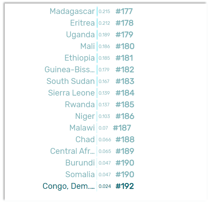
Firstly, we need the first and last entry in the ranking list:
The Democratic Republic of the Congo ranks last with the lowest consumption (rank #192) with 0.02 tonnes per capita.

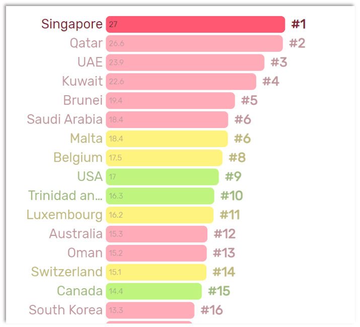
Singapore achieves the highest consumption value with 27 tonnes per capita.

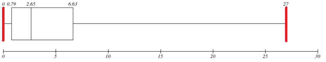
Draw this information in your boxplot:

(Images adapted from https://www.imathas.com/stattools/boxplot.html)

For the median, we need the countries in the centre of the data set:
Rank #96 (Ecuador) with 2.72 tonnes per capita and Rank #97 (Gabon) with 2.58 tonnes per capita.

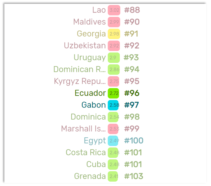
This gives us a rounded median of 2.55 tonnes per capita.

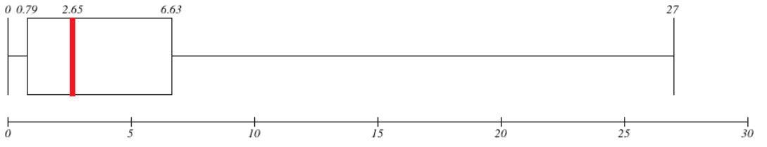
For the first quartile, we need the ranking of the countries in the centre of the first half of the data set:
Rank #144 (Honduras) with 0.839 tonnes per capita and rank #145 (Bangladesh) with 0.745 tonnes per capita.

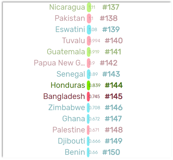
This gives us a rounded first quartile value of 0.79 tonnes per capita.

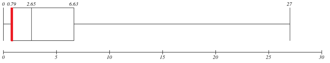
For the third quartile, we need the ranking of the countries in the centre of the second half of the data set:
Rank #48 (France) with 6.65 tonnes per capita and rank #49 (Seychelles) with 6.61 tonnes per capita.

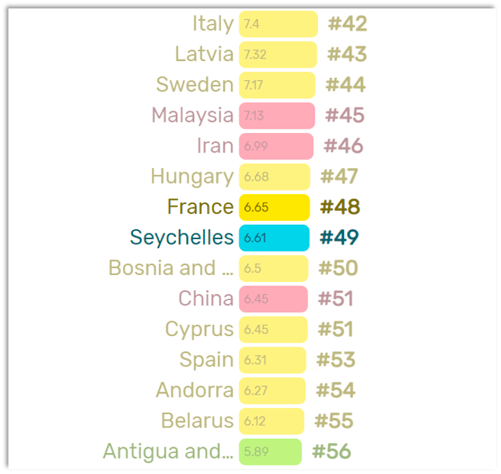
This gives us a rounded third quartile value of 6.63 tonnes per capita.

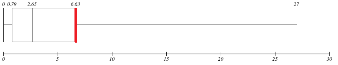
Now we have our boxplot ready!

We can now check whether the carbon dioxide consumption of a particular country is within the limits of the box. The carbon dioxide consumption of Germany with a value of 10.8 tonnes per person is clearly outside the box.

Is your country within the boundaries of the box?