Working with web services

Introduction to Working with Web Services in GIS

In GIS, web services allow users to access and visualize spatial data directly from online sources without the need to download large datasets. These services provide real-time access to high-quality basemaps, satellite imagery, and thematic layers, making them essential for dynamic mapping and analysis.

In this lesson, we will explore how to use different types of web services in GIS applications like QGIS, including:

✅ WMS (Web Map Service) – Loads map images from an online server.
✅ WMTS (Web Map Tile Service) – Provides fast-loading tiled maps for efficient visualization.
✅ WFS (Web Feature Service) – Allows access to vector data that can be queried and edited.
✅ WCS (Web Coverage Service) – Serves raster datasets, such as elevation or climate models.

By the end of this lesson, you will be able to connect to and use web services to load basemaps, display online datasets, and integrate real-time spatial information into your GIS projects—all without downloading any data. We can just load web-based services and then extract those data as .jpeg images, shapefiles or .tiff images, depending on the service type.

Let’s get started with web-based GIS mapping and some definitions first! 🌍🗺️

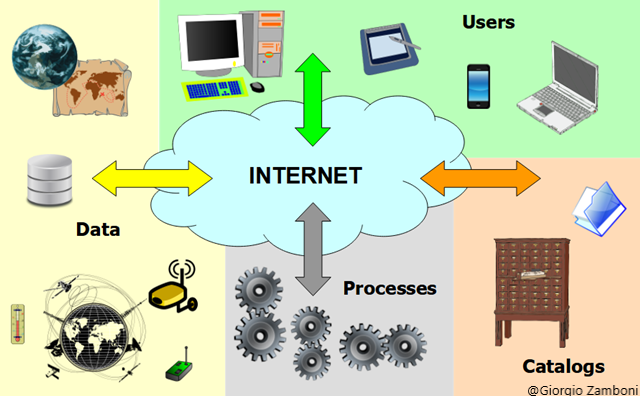
According to the GIS4Schools [1] educational resources, geospatial Web Services and data are stored on servers connected by means of the internet (like the web applications we explored during the first lessons of this course, i.e. the Copernicus Browser, EMODnet etc.). The general concept can be summarised as a distributed GIS (see the image below). We may have geospatial data of every type (maps; aerial, drone, satellite imagery; geolocalized temporal series) stored on distributed servers, we have users who can be equipped with different tools (desktops, laptops, tablets, smartphones, etc). In order to find data we need geospatial catalogues and, if we want also to process data, we may need processing tools, which again stay on distributed servers. The glue of this distributed GIS, which is also called the Geospatial Web, is the internet.

Such a kind of system is based on the concept of Web Service, which is a software system designed to support interoperable machine to machine interaction over a network. As we are dealing with geospatial data, we are interested specifically in Geospatial Web Services, which allow geospatial data and functions to be interoperable.

Interoperability is the capability to communicate, execute programs or transfer data among various systems with different hardware and software platforms, data structures and interfaces in a manner that requires the user to have little or no knowledge of the characteristics of those units and allow the usage of the exchanged information and data without special effort by either system, or without any special manipulation.

In order to obtain interoperability, standards are needed. A distinction can be made between “de facto standards”, which are technical instructions used by a noteworthy number of people and/or organizations and “de jure standards”, which are technical instructions set by national and/or international standardization organizations. In the case of the Geospatial Information Science, we refer to ISO TC 211 Standards and OGC (Open Geospatial Consortium) Standards. OGC Web Services expose geographical functionalities to web users through standard web protocols. The use of the XML (eXtensible Markup Language) allows the encoding of data, rules and functions in a format that is both human-readable and machine-readable.

The functioning of OWS (OGC Web Services) can be summarised in four steps:

• the client contacts the server and queries it about its functionalities;
• the server sends back to the client an XML document containing the functionalities of the supported service;
• the client asks the server for data;
• the server provides the data as requested.

The most important geospatial web services about data are:

• WMS/WMTS (Web Map Service/Web Map Tile Service), which serve map images in a bitmap format (e.g. PNG, GIF, JPEG, etc.) and sometimes also in vector graphics (points, lines, curves and text, which can be expressed in formats like SVG). The WMTS is an extension of the WMS which alleviates the CPU intensive on-the-fly rendering problem when transferring massive amounts of data by using pre-rendered map tiles.
• WFS (Web Feature Service), which offers direct access to vector geographic information at the feature and feature property level, where a feature represents a physical entity, e.g. a building, a street, etc. Data is generally transferred in an XML-based GML format, but other formats like shapefiles can also serve for transport.
• WCS (Web Coverage Service), which supports requests for coverage data (gridded and raster data). While a WMS returns only an image, the results of a WCS can be used for modelling and analysis. WCS also allows more complex querying, for instance only the extraction of a portion of the data.

Accessing OGC services with QGIS

QGIS allows the connection to servers offering geospatial data in compliant with the OGC service standards. Let’s continue with our QGIS Project ‘GIS_Training’ data. In case you closed QGIS, let’s open it again and load our saved ‘GIS_Training’ project and the Cyprus data!

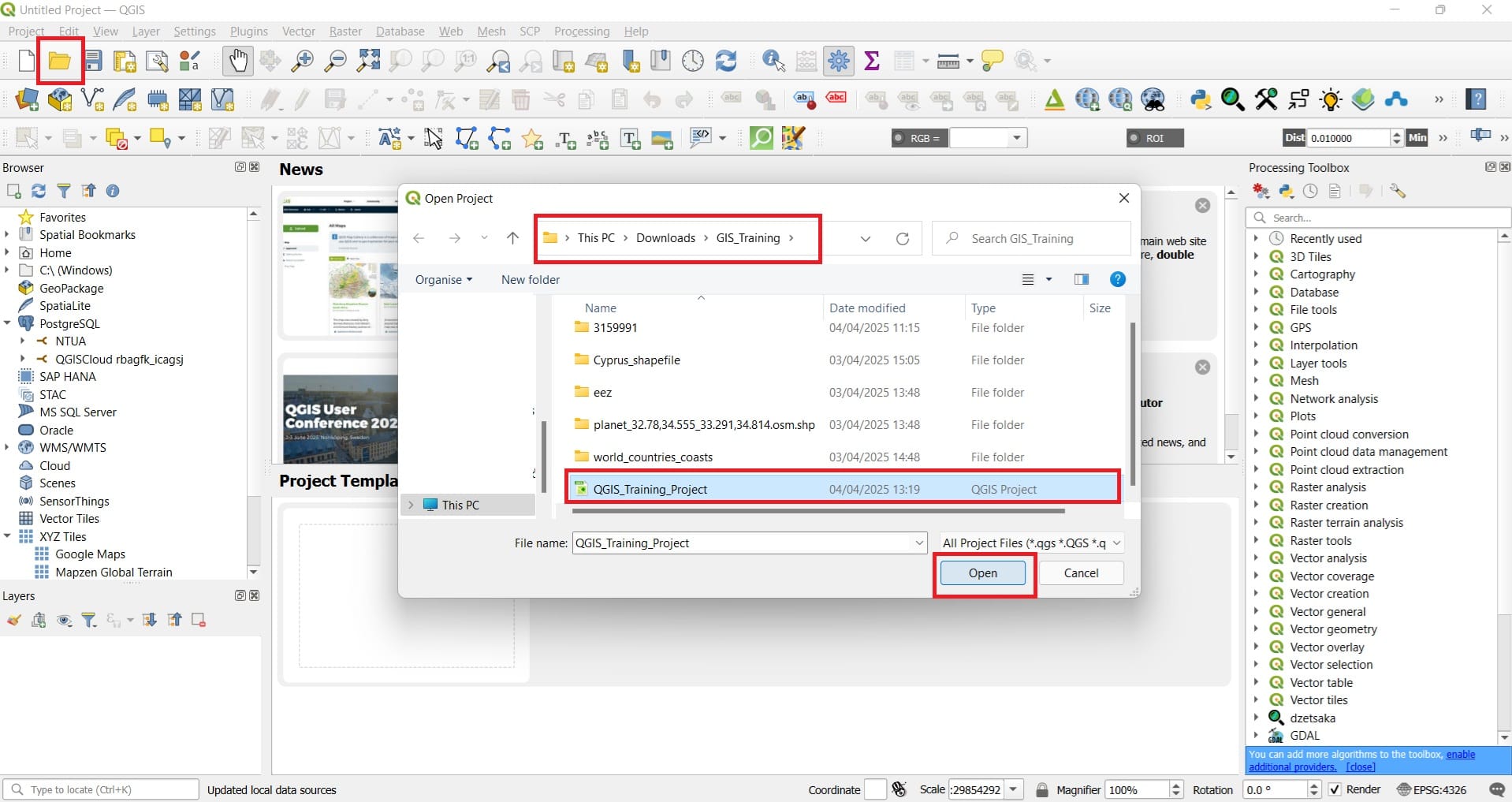
In the ‘Main Toolbar’ we select the ‘Folder’ icon > Browse to your ‘GIS_Training’ folder > Select the ‘QGIS_Training_Project’ > Open

Let’s try now to load different web services from different web repositories, for example, OpenStreetMap WMS – by terrestris (WMS), the EMODnet Web Services (WMTS & WFS). The links we are going to use are the following:

1. 1. OpenStreetMap WMS – by terrestris (WMS): http://ows.terrestris.de/osm/service
   2. EMODnet Web Services (WMTS & WFS): https://ows.emodnet-bathymetry.eu/wms or https://ows.emodnet-bathymetry.eu/wfs

 

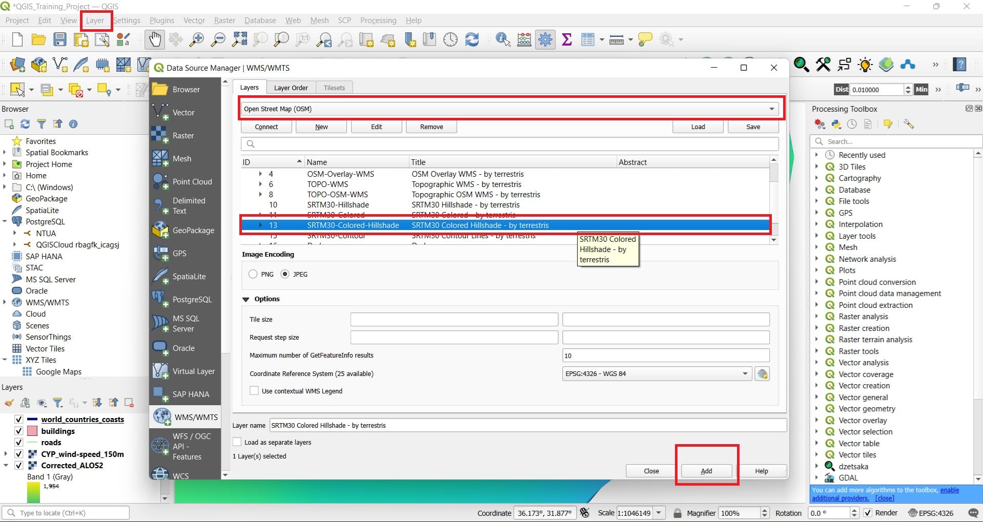
Step 1: In order to load our first WMS service, we select (similarly to the shapefiles and raster data) on the Main Toolbar > ‘Layer’ > ‘Add Layer’ > ‘Add WMS/WMTS Layer’.

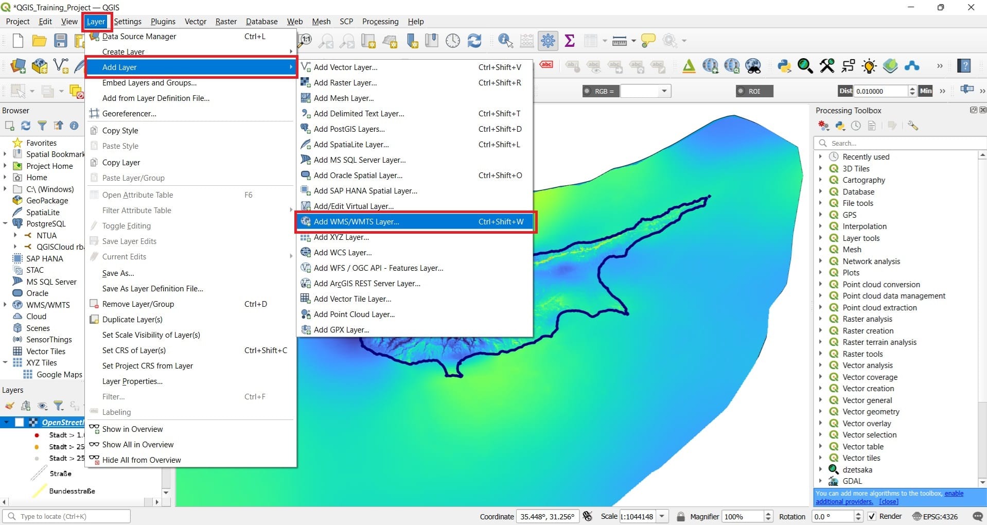
Then, a new window will pop-up, the ‘Data Source Manager WMS/WMTS’ (on the background on the photo below) and we select > ‘New’ to establish a new connection with the server.

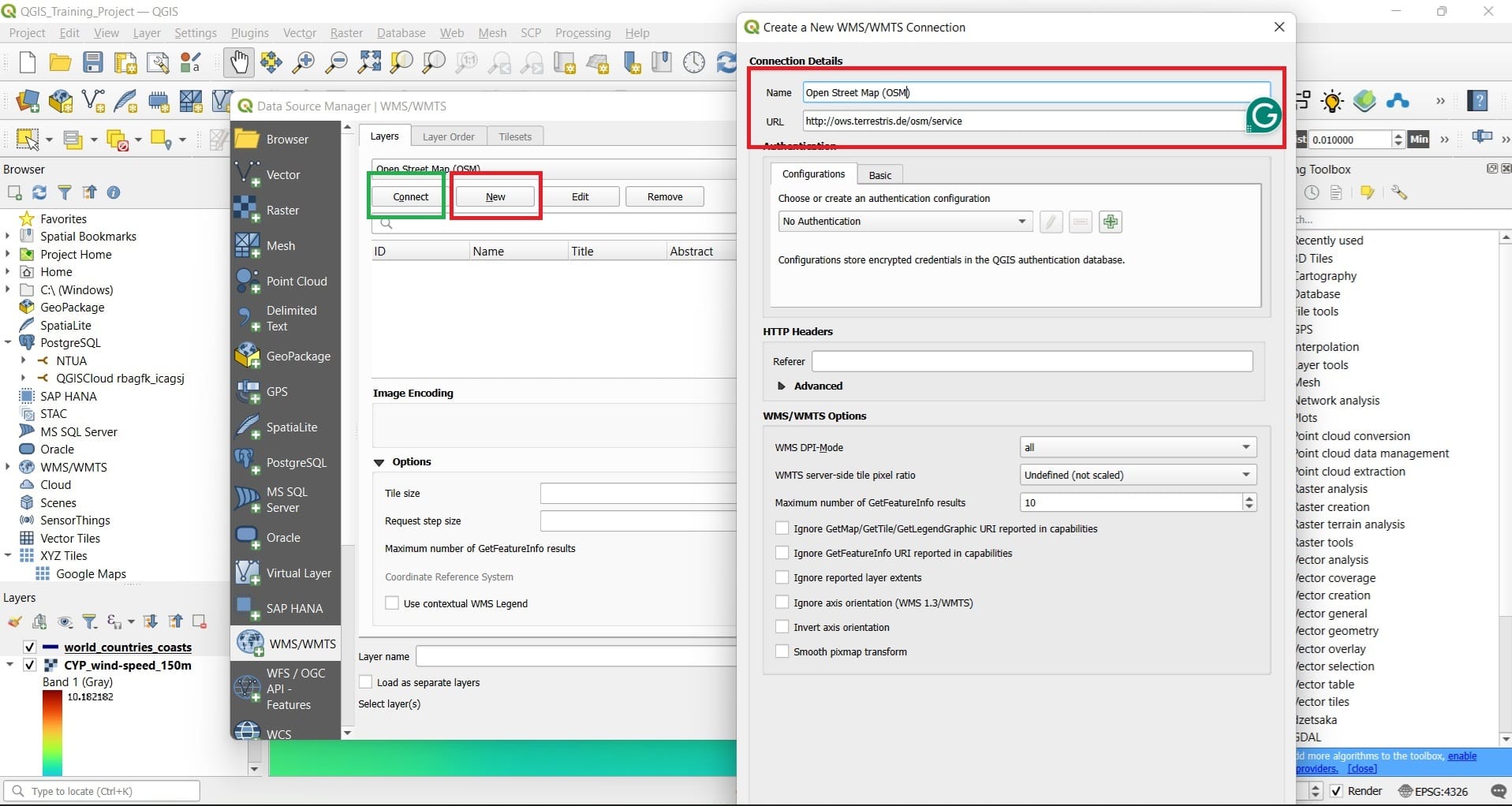
In the ‘Create a New WMS/WMTS Connection’ window we should only give the name of our connection, i.e. ‘Open Street Map (OSM)’ and then under the ‘URL’ window to copy and paste this link  http://ows.terrestris.de/osm/service.

Then we press ‘Ok’ AND ‘Connect’ (green box on the background window) in order to see the files inside the OSM web services

After we press ‘Connect’, we will see the following list of data.

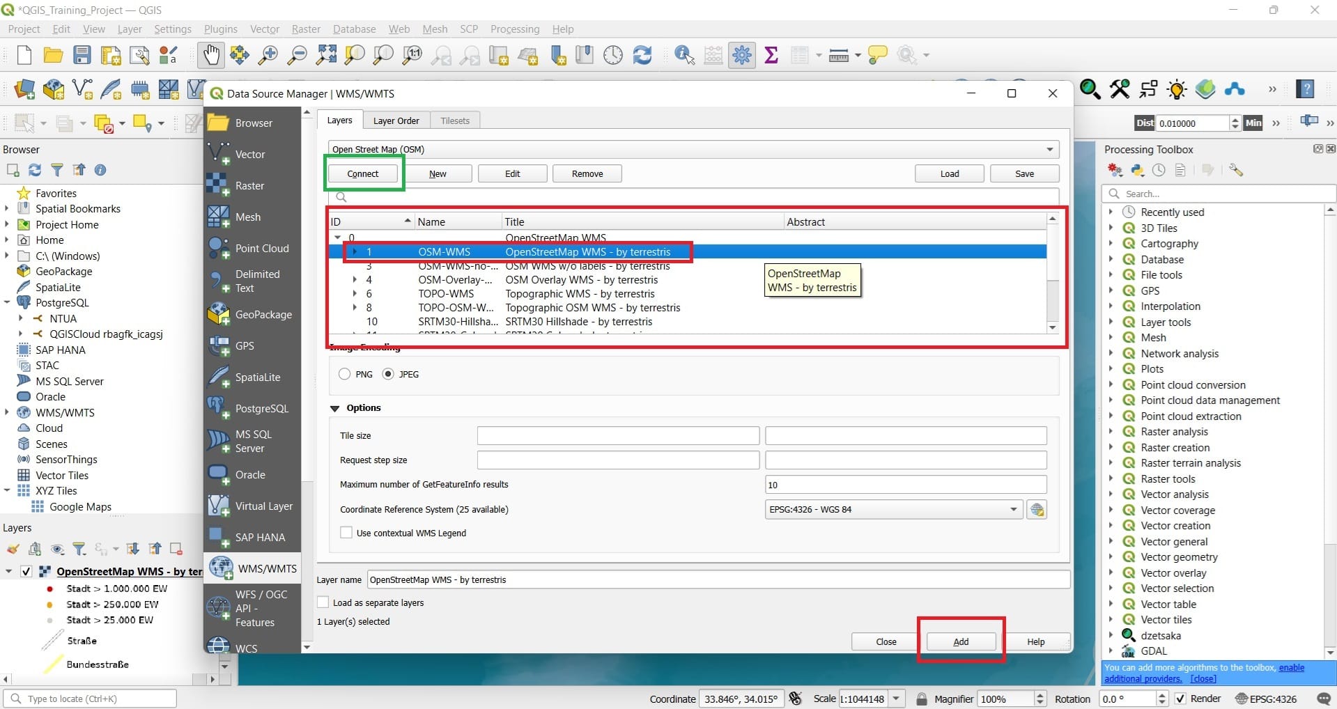
We can now select option number 1 (OSM-WMS, OpenStreetMaps WMS – by terrestis) and then > Press ‘Add’

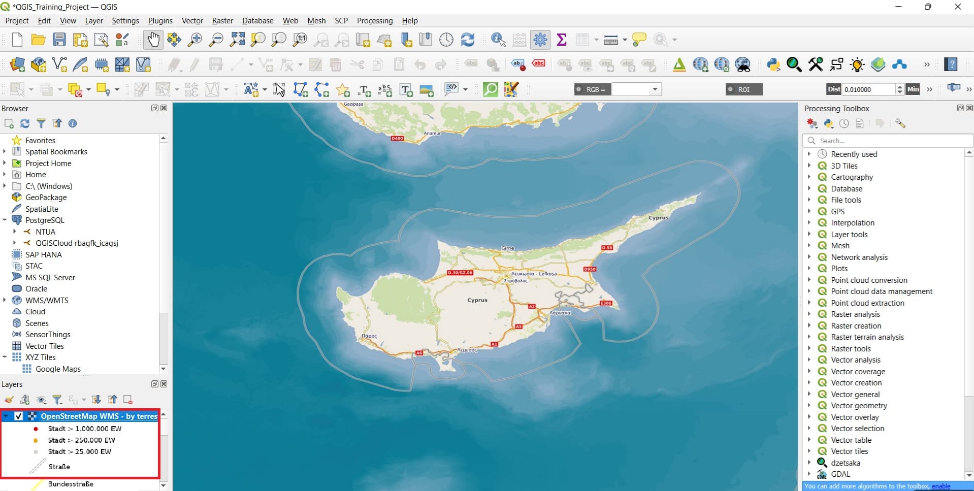
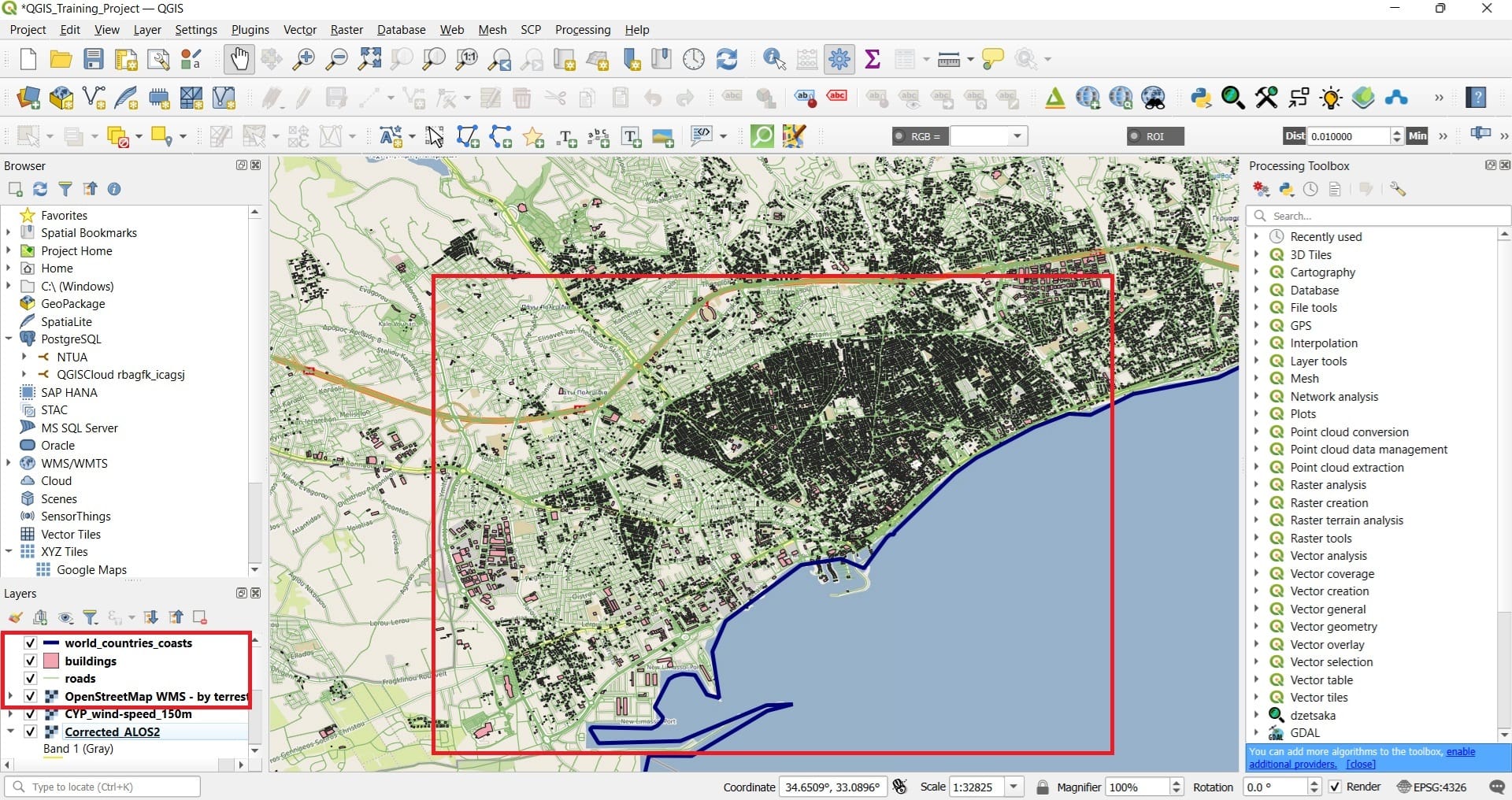
Don’t get confused! The shapefiles and raster images we loaded in the previous lessons are still there. You can just bring on top the Cyprus coastline like we did previously. The main reason we don’t see the vector and raster files is because WMS services bring images (rasters actually) so, they ‘cover’ our datasets because they have a global coverage!

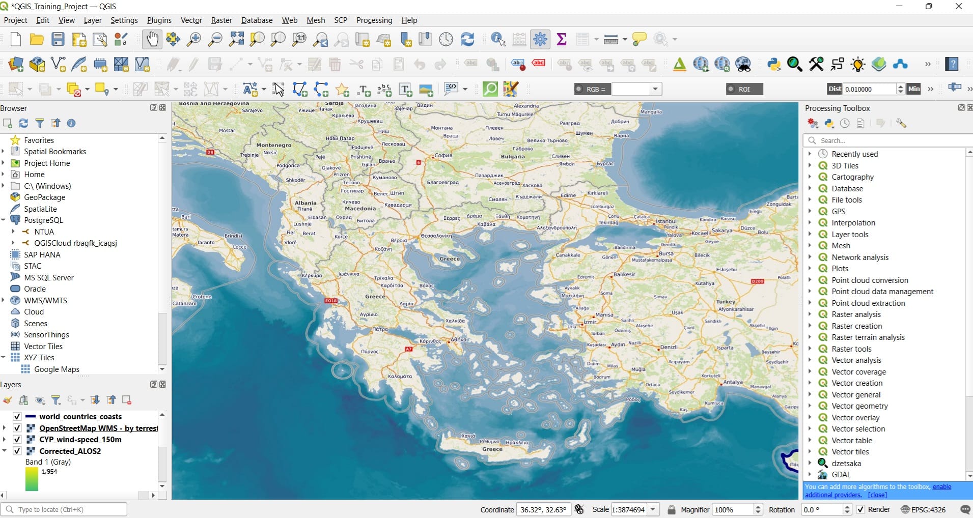
You can also zoom-out and zoom-in in other areas or countries, for example, in Greece!

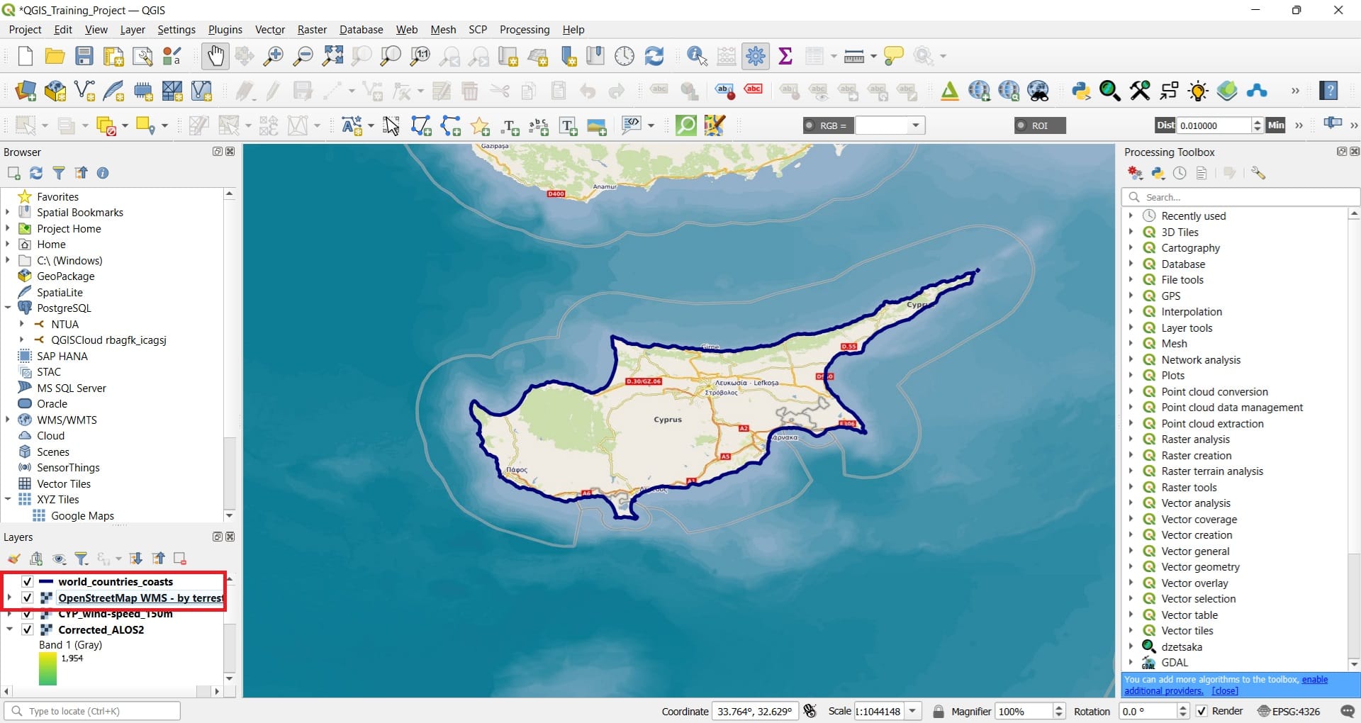
But, let’s go back to Cyprus and let’s zoom-in in Limassol area. If we also move on top the buildings and/or the roads shapefiles we had downloaded in the previous lessons, you may see the Open Street Map (OSM) WMS and on top all the shapefiles we have downloaded.

We can also explore the differences between the actual shoreline (from the Open Street Maps WMS) and the shoreline we have downloaded. Why we see those differences? It is always a matter of accuracy! If we extracted the shoreline using old satellite images with a low spatial resolution, the coastine won’t be that accurate. Also, if a geographer or a GIS Analyst digitized the shoreline by hand, it is always a matter of what basemaps she/he used to digitize the shoreline!

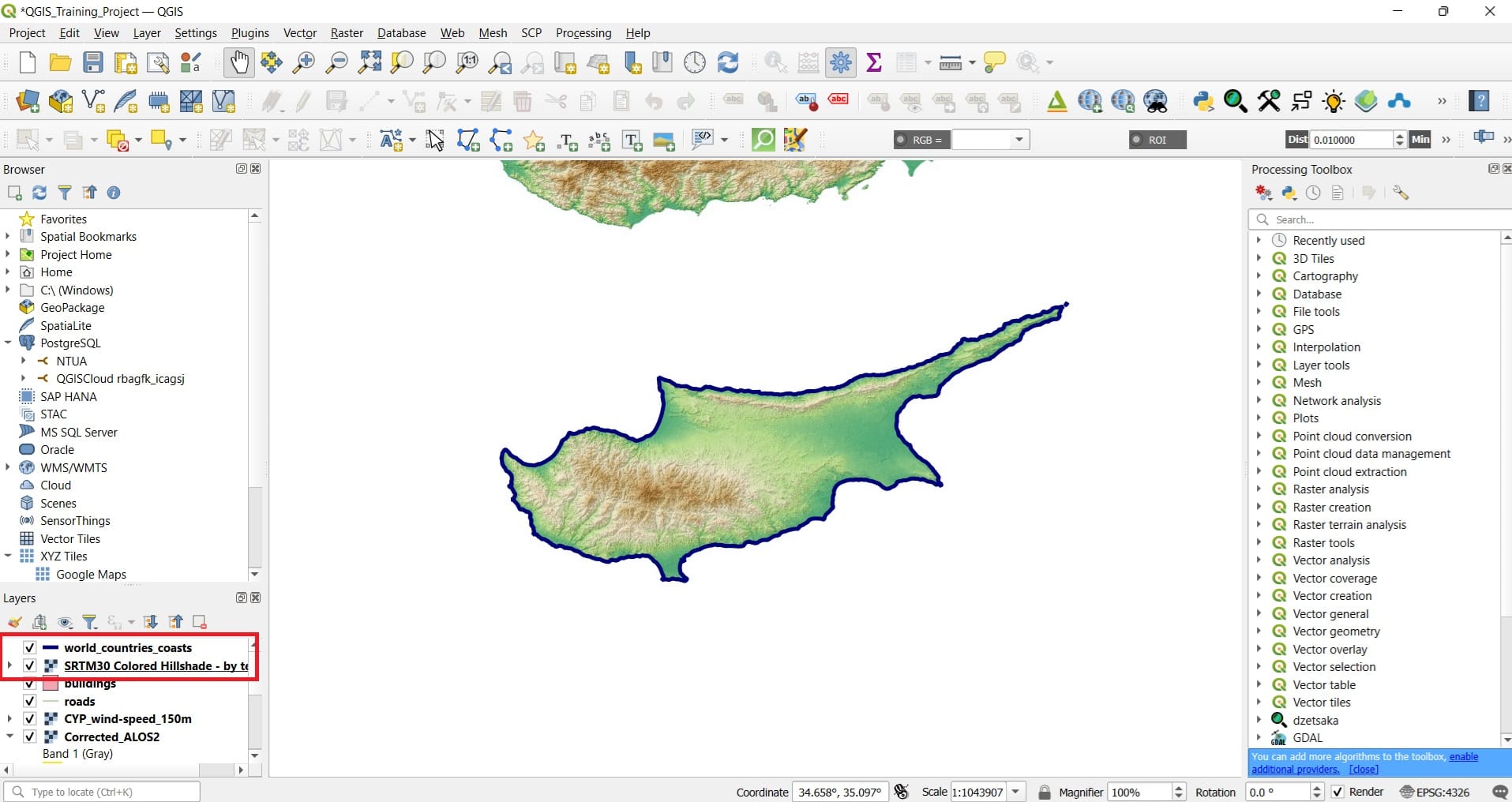
You may also experiment and add more layers from the OSM WMS Services, like number 13, the SRTM30-Colored-Hillshade (the NASA Shuttle Radar Topography Mission – SRTM). It is pretty similar to the Digital Elevation Model (DEM) we have downloaded in the previous course but, with a huge difference! The OSM WMS Service is an image and the DEM we have downloaded is a .tiff georeferenced image that can be processed! We will explain why is that important in our next course!

The SRTM30 result! Why SRTM30? Because the size of each pixel, as can be seen from the satellite, it’s 30 meters! The DEM we have downloaded has a spatial resolution (cell/pixel size of 25 meters)

Let’s try to load some shapefiles from Web Services like the EMODnet WFS!

Step 2: In order to load our first WFS service, we select (similarly to the shapefiles and raster data) on the Main Toolbar > ‘Layer’ > ‘Add Layer’ > ‘Add WFS / OCG API – Feature Layer’.

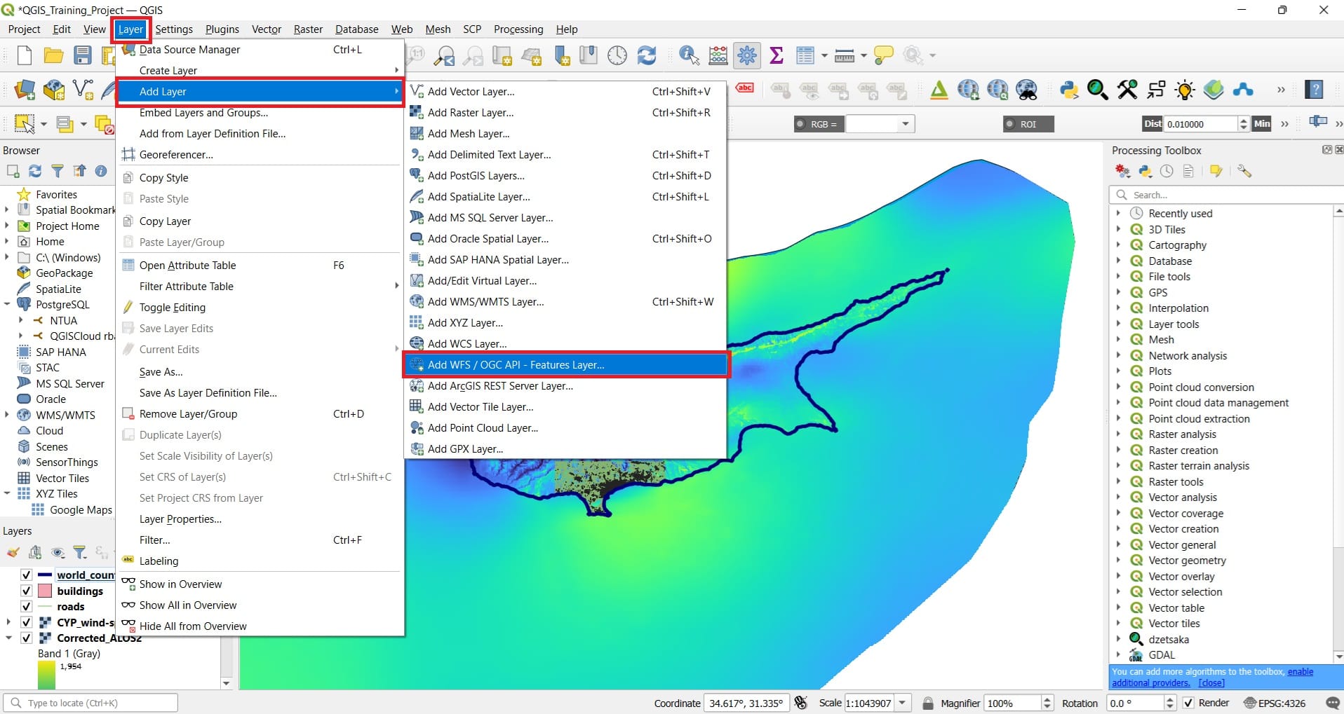
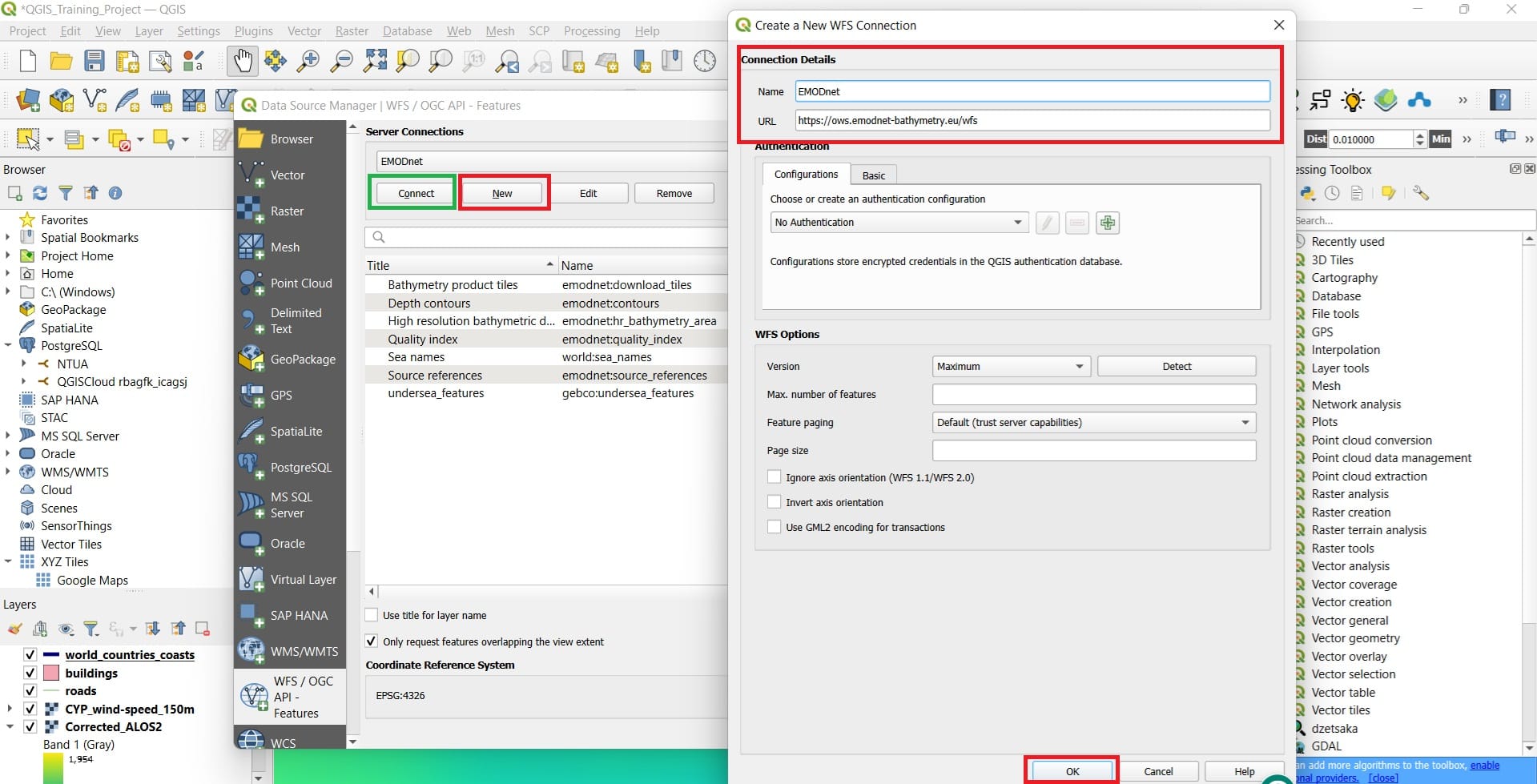
In the exact same way like in the WMS/WMTS Services, a new window will pop-up, the ‘Data Source Manager WFS / OCG API – Feature’ (on the background on the photo below) and we select > ‘New’ to establish a new connection with the server.

In the ‘Create a New WFS / OCG API – Feature Connection’ window we should only give the name of our connection, i.e. ‘EMODnet’ and then under the ‘URL’ window to copy and paste this link  https://ows.emodnet-bathymetry.eu/wfs.

Then we press ‘Ok’ AND ‘Connect’ (green box on the background window) in order to see the files inside the EMODnet web services.

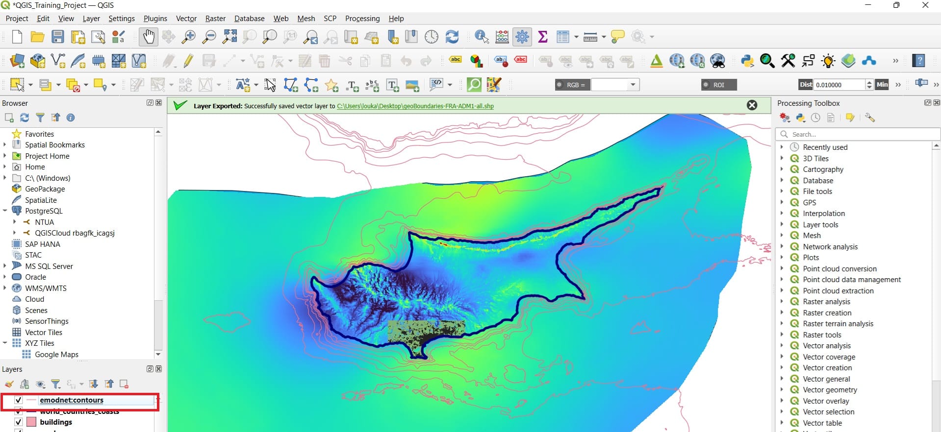
This time, we can load the bathymetric contours, not only for Cyprus but, for entire Europe. We just select the ‘Depth Contours’ layer and then, press ‘Ok’. Keep in mind that we can directly process the contours dataset, we can clip only the contours of Cyprus or we can export the entire dataset as a shapefile in our computer. However, we will test those capabilities in our next lessons. The result of the contrours shapefile will look like this.

IMPORTANT NOTE: The WFS (shapefile) data we loaded, is not directly saved to our computer! If we want to save the ‘contour’ data, we right-click on the file (Layers browser) > ‘Export’ > ‘Save as feature layer’. 

We may also save a WMS or WMTS file as a georeferenced image but, it’s a bit more complex. However, you can create Map Layouts using the WMS/WMTS services. Check the Cartography and Spatial Thinking course on how to do that!

✅ Wrapping Up: Introduction to Working with Web Services in GIS

You’ve now completed the course on Working with Web Services in GIS—a vital step in expanding your skills with real-time, online geospatial data. Throughout this lesson, you explored how to connect to and work with a variety of services such as WMS, WMTS, WFS, and WCS, each offering unique capabilities for loading maps, vector features, and raster datasets directly into QGIS. You’ve seen that there’s no need to download large files when different services allow you to visualize, explore, and even extract the data you need on demand. These skills are especially useful in educational and classroom settings where quick access, flexibility, and lightweight processing are key.

In the next course, we’ll dive into Processing Tools and Plugins in QGIS, where you’ll learn how to transform and analyze both vector and raster data with powerful built-in tools and additional plugins designed to enhance your spatial workflows.

Great job—and get ready to unlock the full analytical potential of QGIS in your classroom or projects! 🗺️🧩🚀

Useful links

1. GIS4Schools: Introduction to Geospatial Web Services
2. OGC – WMS/WMTS: Web Map Service / Web Map Tile Service
3. OGC – WFS: Web Feature Service
4. OGC – WCS: Web Coverage Service
5. Services – WMS: OpenStreetMap WMS – by terrestris (WMS)
6. Services – WMTS – WFS: EMODnet Web Services (WMTS & WFS)
7. Copernicus Web Services (WCS)