The QGIS Platform

Introduction

In this lesson, we will walk you through the process of downloading and installing QGIS Desktop on your computer and your school’s lab. QGIS is a powerful, free, and open-source Geographic Information System (GIS) that enables educators and students to explore, analyze, and visualize spatial data.

By the end of this lesson, you will be able to:

✅ Locate the official and most reliable source for downloading QGIS.
✅ Identify the system requirements needed for a smooth installation.
✅ How to install QGIS Desktop on Windows, macOS, and Linux.
✅ Set up QGIS in a school lab environment for classroom use.
✅ Navigate the QGIS interface, install plugins, and load basemaps.

✅ Learn how to identify the CRS of a dataset in QGIS.
✅ Reproject vector and raster data into a different CRS when needed.
✅ Set and manage the project CRS to ensure consistency across layers.

Let’s get started with the installation and prepare for hands-on GIS learning!

Step 1: Visit the official QGIS page for downloading the .exe file (link)

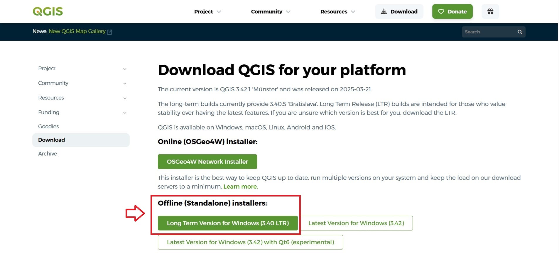
Press the green tab ‘Long Term Version for Windows (3.40 LTR)’ under the Offline (Standalone) installers and the .exe download will start! It might take some time so, be patient!

Step 2: Run the .exe file

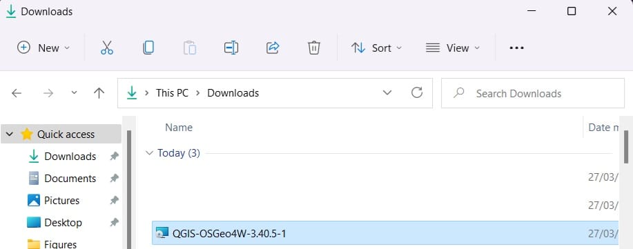
Navigate to your ‘Downloads’ folder and double-click the ‘QGIS-OSGeo4W-3.40.5-1’ .exe file. The installation will start and then you press ‘Next’ > ‘Accept the terms in the Licence Agreement’ and ‘Next’ > ‘Next’ > ‘Install’ > ‘Yes’ to the installation pop-up window. It will also take some time!

After the installation is completed, a new folder ‘QGIS 3.40.5’ will be created on your Desktop and either via the folder or the Windows start button (see the Image below) you can now open QGIS Platform.

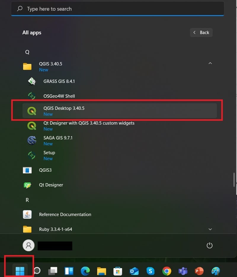
It will still take some time while loading for the very first time since it’s installing some Python libraries on your computer (it is completely safe! such applications need programming languages to run in the background processes.)

Step 3: That was it, WELCOME TO THE GIS WORD (ok, not yet, but, that was a first important start!). The QGIS interface will look like the image below:

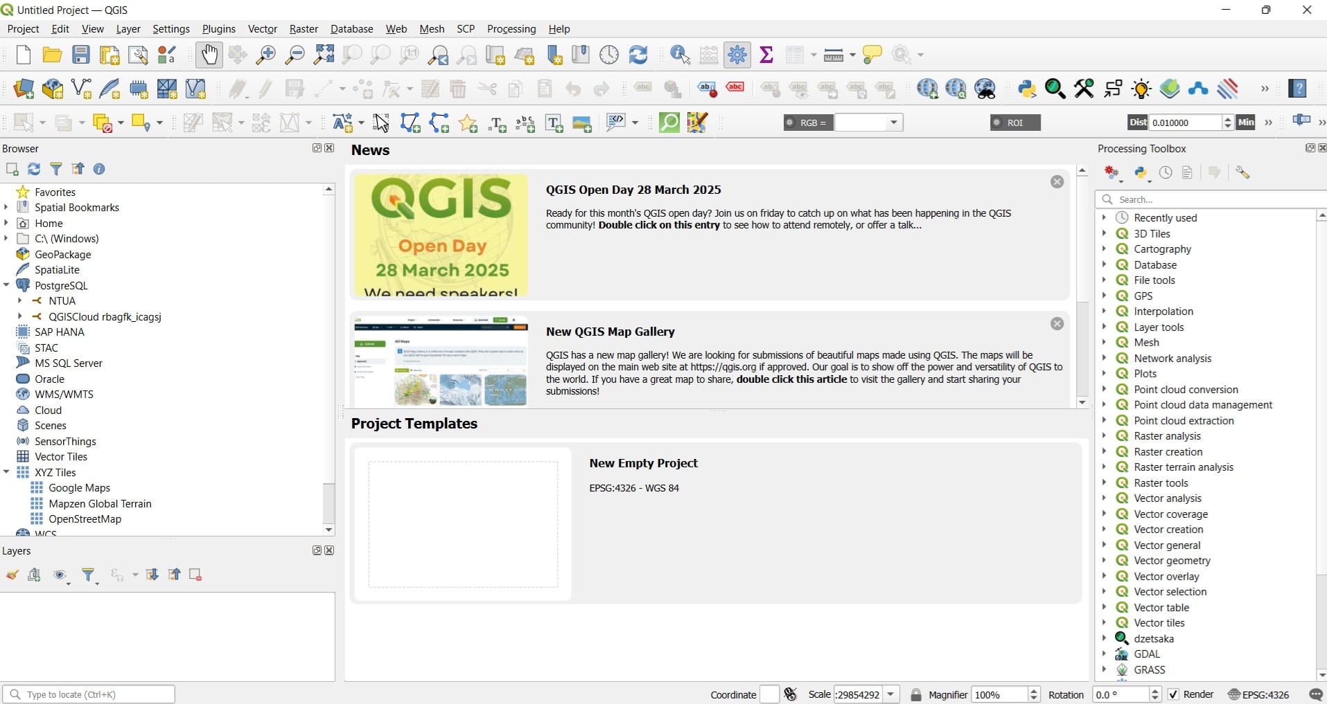
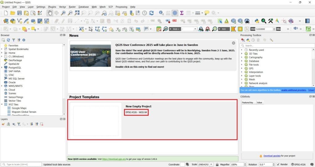
Step 4: What is our goal? To create our first project. So, let’s click the ‘New Empty Project’ template under the ‘Project Templates’!

Step 5: Let’s save our project using the ‘Floppy Disk’ icon or navigate to the main toolbar on the top left corner and press ‘Project’ > ‘Save as’ and save your project.

IMPORTANT: Try to save your projects and the data you are downloading (we will work on that during the next lesson) under folder C:. For example, create a new folder on your C:\ drive called ‘GIS_Activitites’ and from now on, you can work all your projects from this folder. Why we do this? Because GIS and the programming languages like Python working on the background are struggling some time with the directories/paths to identify our projects or data due to the special characters (i.e. %,&,*,£) or with other language letters! Thus, we need our directories to be short, simple and with as less special characters as possible!

Step 6: Let’s explain the main toolbars, dialog boxes and browsing options of QGIS interface. This will make our life easier within the next steps and lesson for GIS and Earth Sciences course!

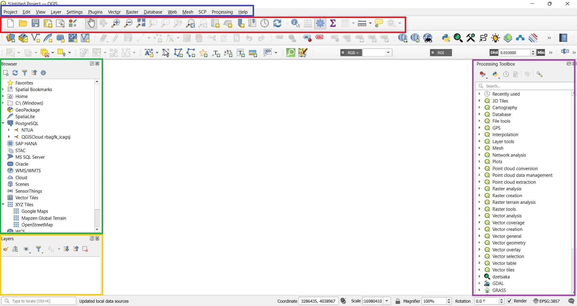
In the Blue Box, we see the QGIS Main Toolbar which is the most important feature of QGIS Interface. Everything we need is there! In particular:

• Under the ‘Project’ button, we may save our Project, we may change our Project Properties or we may create a layout to export our first maps!
• Under the ‘Layer’ button, we may add any type of geospatial data (vector or raster, see the previous lesson!) or we can create a new empty spatial dataset (mainly a vector dataset).
• Under the ‘Plugins’ button, we may install new libraries/tools on the QGIS interface. But….wait, what is a Plugin? Plugins in QGIS add useful features to the software. Plugins are written by QGIS developers and other independent users who want to extend the core functionality of the software. These plugins are made available in QGIS for all the users.
• Under the ‘Vector’ and ‘Raster’ buttons, we may find all necessary processing tools either for vector or raster spatial data (we will work on that during our next lesson!).
• Under the ‘Web’ button, we can load and connect online services and spatial data like Open Street Maps (OSM) or satellite images.
• Under the ‘Processing’ button, is the main element of the processing interface (Purple Box), and the one that you are more likely to use for developping an activity.

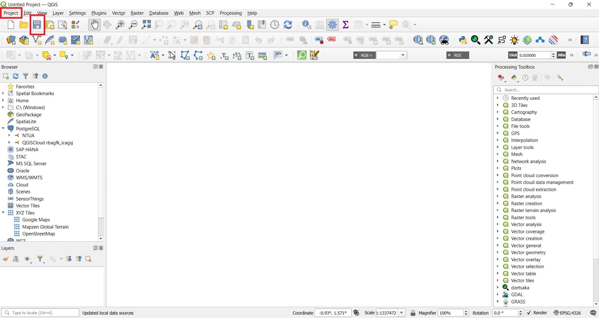
In the Red Box there are mainly options and buttons related to the main QGIS drawing area (White box in the middle of the screen). These tools include:

• Create new project, open an already existing one or save current project (the first 3 icons).
• With the ‘Hand’ icon you may move the map
• With the ‘Magnifying glass’ icons you can zoom-in and zoom-out.
• At last, with the ‘Gear wheel’ you can re-open the processing toolbox on the right side (Purple box) and,
• With the ruler you can measure distances.

In the Green Box you may nagigate to your computer folders, load spatial data with the drag and drop option, create new spatial data or connect to different online services. Thus, there are 2 options to load spatial data! Either via the drag and drop method directly from our folder (Green Box) or via the ‘Layer’ option on the main toolbar (Blue Box).

In the Yellow Box we see all data we are loading (see the OSM example below). We can hide different layers by unchecking the visibility box or we can change the drawing order of our layers, i.e. which one is shown on top etc. To do that, we can simply click a layer and drag it up or down in the table of contents (Yellow Box).

In the Purple Box we may find all processing tools that are already installed in the QGIS platform. We can also use the ‘Search’ bar. But, can we also find other toolboxes that are not installed? The answer is ‘Yes’, if we first install them via the ‘Plugin’ button on the Main toolbar (Blue box). We will follow the step-by-step process within the next lessons!

Setting up a CRS in QGIS Platform

​Step 7: Before starting any GIS project, it’s essential to verify the Coordinate Reference System (CRS) of your data. The CRS defines how your two-dimensional, projected map in your GIS relates to real places on the earth. ​

Commonly, datasets you download are in the WGS 84 (EPSG:4326) geographic coordinate system, which uses degrees of latitude and longitude. Additionally, some datasets, especially those from European sources, may use projected coordinate systems like ETRS89 / LAEA Europe (EPSG:3035) or ETRS89 / UTM zones. ​Basemaps, such as those from OpenStreetMap or Google Maps, typically use the WGS 84 / Pseudo-Mercator projection (EPSG:3857) [9].

When we load QGIS platform and we create a new project, there is the option to set the pre-define Geographic Coordinate Systmem WGS ’84 (EPSG: 4326).

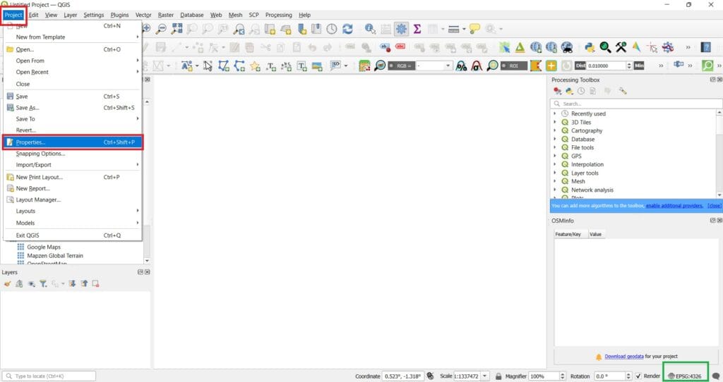
To ensure spatial accuracy and proper alignment of your data layers (we will download different vector and raster datasets in the upcoming lesson), it’s crucial to set your QGIS project’s CRS to match the CRS of your primary dataset. In QGIS, you can set the project’s CRS either by clicking on the CRS indicator in the bottom-right corner of the window (green box on the image below) or by selecting ‘Project’ on the main QGIS toolbar > ‘Properties’ > ‘CRS’. ​

With both options, a new window will pop-up (see image below) where we can set the CRS of our preference!

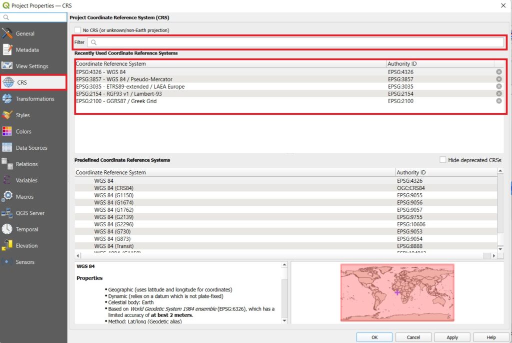
On the ‘Filter’ window, we can search for different geographic or projected coordinate systems either by typing the name (i.e. ‘Greek’ or ‘GGRS87’) or the EPSG code (i.e. ‘2100’ for the Greek projected coordinate system). 

Every time you are using a CRS, it is saved/stored in the ‘Recently Used Coordinate Reference Systems’ and it’s easier to set-up the CRS of our preference.

QGIS also supports “on-the-fly” CRS transformation, allowing layers with different CRSs to be reprojected dynamically to match the project’s CRS. For example, you might get a vector layer showing the boundaries of South Africa projected in UTM 35S and another vector layer with point information about rainfall provided in the geographic coordinate system WGS 84. In GIS these two vector layers are placed in totally different areas of the map window, because they have different projections. To solve this problem, many GIS platforms include a functionality called on-the-fly projection. It means, that you can define a certain projection when you start the GIS and all layers that you then load, no matter what coordinate reference system they have, will be automatically displayed in the projection you defined. This functionality allows you to overlay layers within the map window of your GIS, even though they may be in different reference systems. In QGIS, this functionality is applied by default [3].

However, for consistency and to minimize potential errors, it’s advisable to reproject your layers to a common CRS when possible. We will work on different reprojection tools for vector and raster datasets in the upcoming lessons.

By verifying and setting the appropriate CRS at the beginning of your project, you ensure that all spatial analyses and map outputs are accurate and reliable!

Step 8: Let’s load our first datasets!

A first option when we open QGIS Platform is to load spatial data already existing in the QGIS installation forlders! Let’s try it. We open the QGIS and we see the following window..

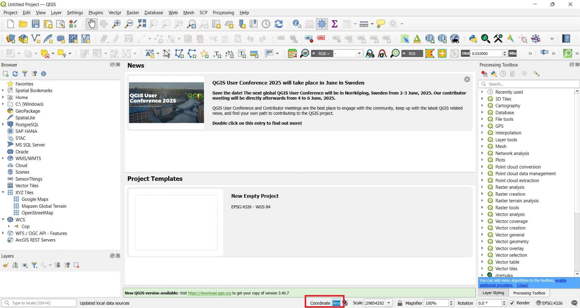
At the bottom of the QGIS interface we see the ‘Coordinate’ tab. If we type ‘world’ and we press enter, a vector layer (shapefile) including all country boundaries as polygons will appear like in the image below.

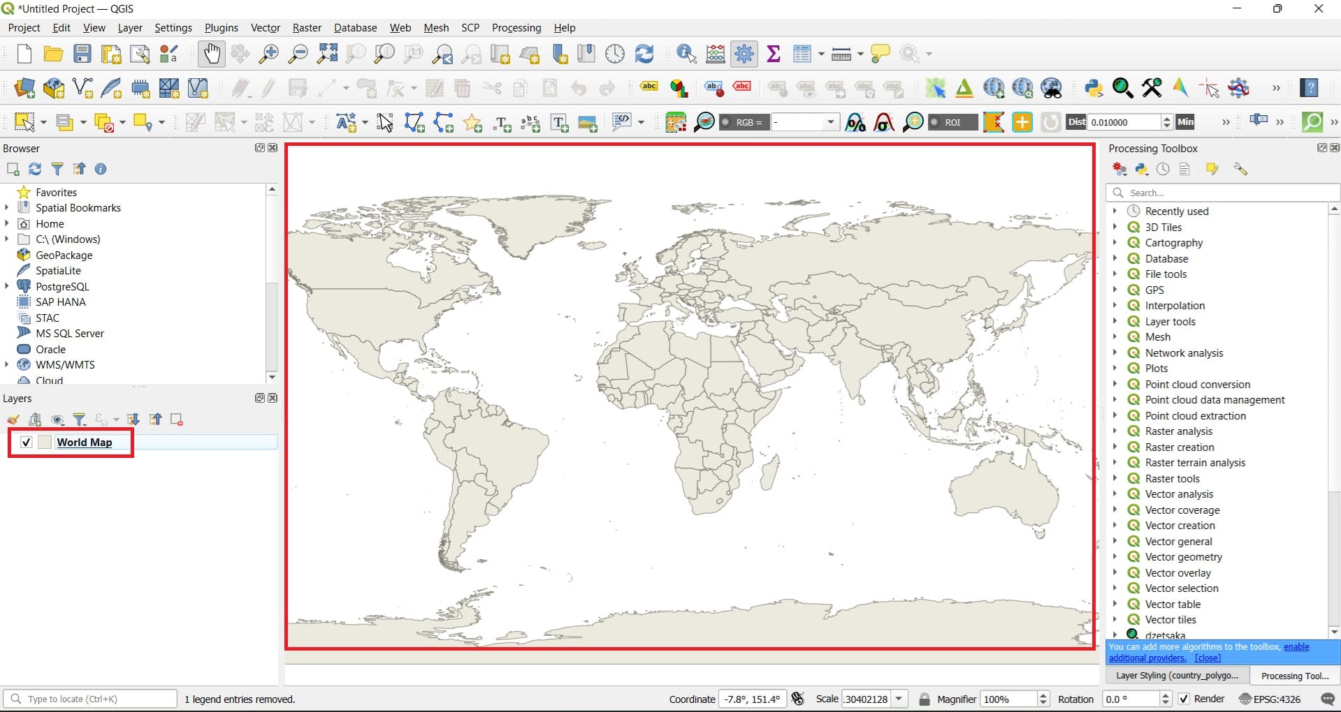
Since our computer has an internet connection, we can directly load some basemaps. Let’s try to load Open Street Maps (OSM). One option is via the ‘XYZ Tiles’ on the ‘Browser’ window > we select the ‘OpenStreetMap’ file and we drag and drop on the ‘Layers’ tab.

And the result will look like….

Another option is to load OpenStreetMap data via the ‘QuickMapServices’ plugin but, this is some we will explore in the upcoming lessons. For now, you may select the ‘Plugins’ button on the main QGIS toolbar (on top) > ‘Manage and install plugins’ > type ‘QuickMapServices’ and select ‘Install’ on the plugin window.

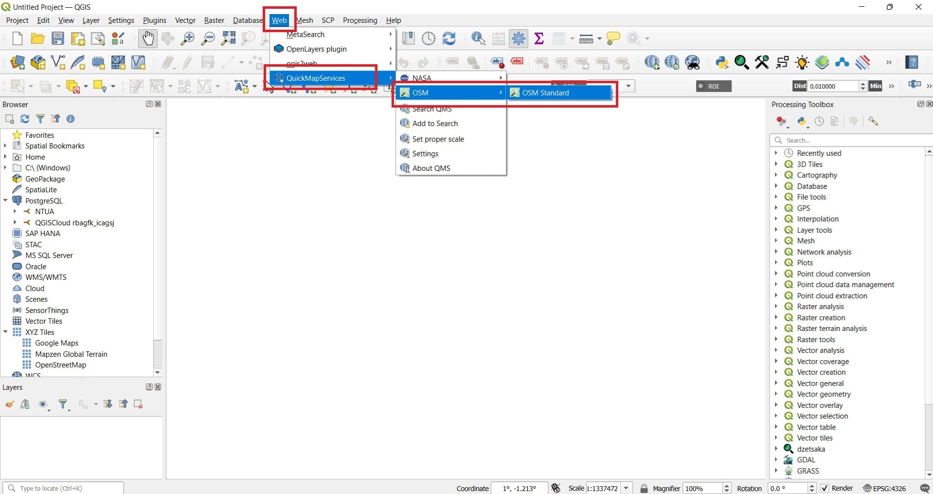
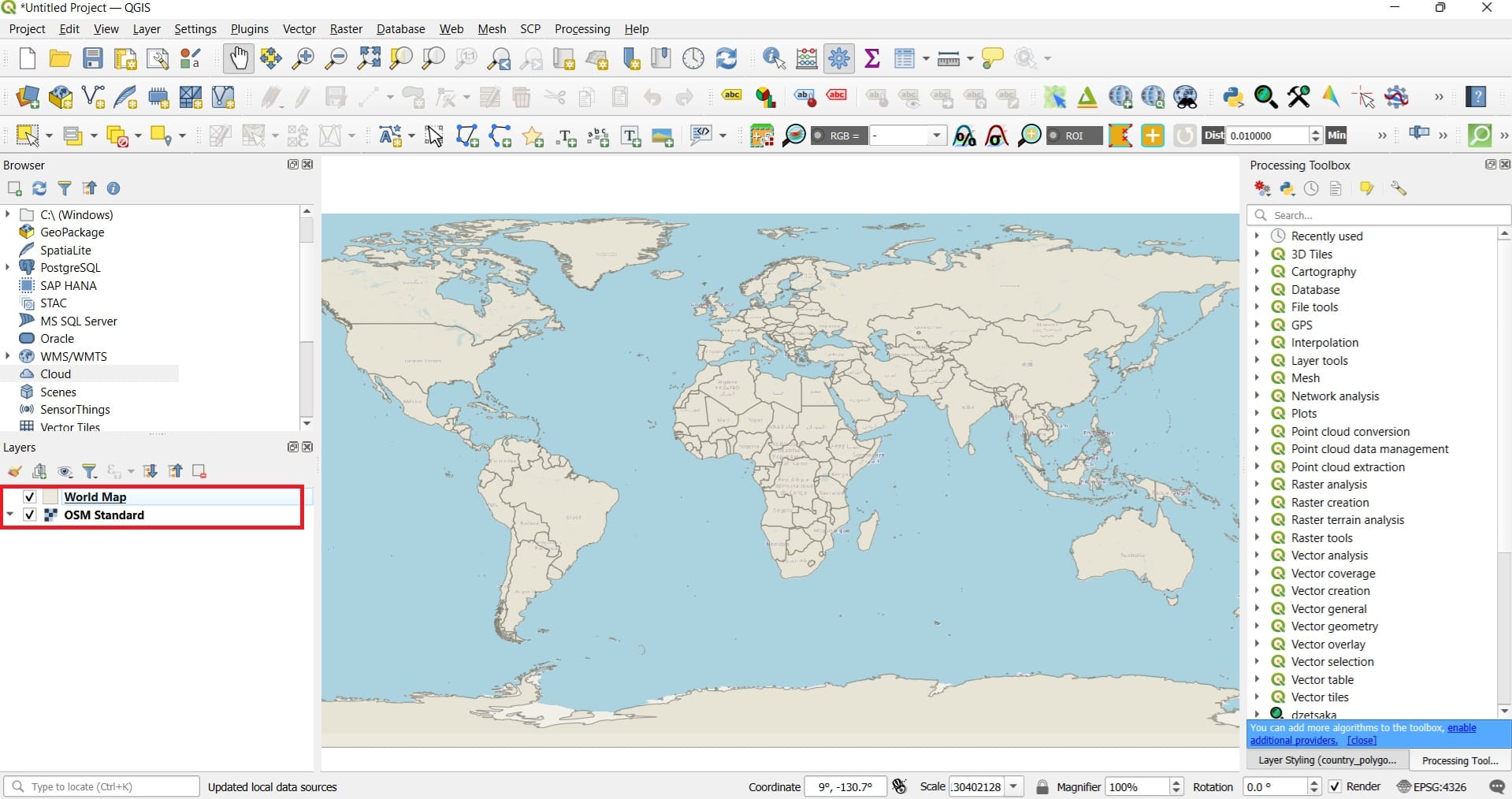
After you install the plugin, navigate to the main toolbar on the top of QGIS interface and press ‘Web’ > ‘QuickMapServices’ > ‘OSM’ > ‘OSM Standard. Alternatively, you may select other basemaps from ‘QuickMapServices’ or the ‘OpenLayersPlugin’.

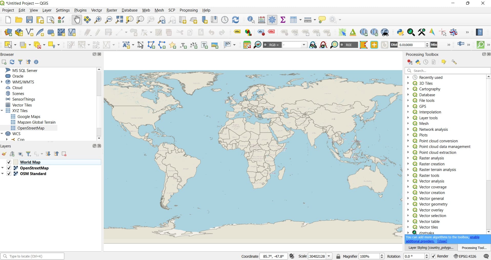
Thist will be the result! We have now loaded Open Street Maps layer and we can zoom-in or zoom-out using our cursor to identify different areas worldwide. Check on the bottom right corner! What CRS is used? It’s EPSG: 4326 – WGS 84 which is a geographic coordinate system. However, we can change it!

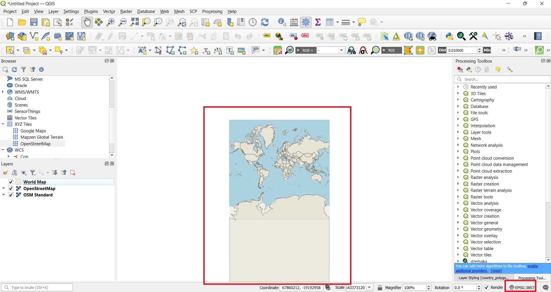
We may try a projected CRS, for example, EPSG: 3857 – WGS 84 Web Mercator or Pseudo Mercator which is a projected coordinate system commonly used for online maps, including OpenStreetMap (OSM). Do you see how the countries and continents sizes changed?

When switching from EPSG:4326 to EPSG:3857, the noticeable changes in the size and shape of continents and countries are due to differences in how each coordinate reference system (CRS) represents the Earth. EPSG:4326 is a geographic CRS that uses latitude and longitude based on a spherical model of the Earth (WGS84), as we explained in the previous lessons. It preserves the actual proportions of geographic features and is ideal for global-scale data, but it does not project the Earth onto a flat surface, which makes it less suitable for detailed mapping or measuring distances.

On the other hand, EPSG:3857, is a projected CRS commonly used in online mapping platforms like Google Maps and OpenStreetMap. It projects the curved surface of the Earth onto a flat plane, preserving angles and shapes locally but distorting areas, especially near the poles. This is why countries like Greenland and Canada appear much larger than they actually are, while equatorial regions like Africa appear comparatively smaller. This distortion is a result of the mathematical transformation used in the Mercator projection, which stretches the map increasingly as you move away from the equator.

Now that we tested our CRS knowledge and the differences, the main question is……Can we overlay other data on top of the Open Street Map layer? Of course we can! Let’s find out in our next lesson related to the online data repositories and how we can download spatial data either in vector or raster format.

Useful links

1. QGIS Beginner Part 1: Making Your First Map