Download raster data

Introduction to Downloading Raster (Gridded) Data

In GIS, raster data represents geographic information as a grid of pixels, making it ideal for elevation models, satellite imagery, land cover maps, and climate data. One of the most common formats for raster data is GeoTIFF (.tiff), which preserves spatial reference information and is widely used in GIS applications like QGIS.

In this lesson, we will explore how to find and download raster datasets from reliable online sources. You will learn how to identify datasets relevant to your project, download them in the correct format, and prepare them for visualization and analysis in GIS software. Understanding how to access and work with raster data is essential for environmental monitoring, spatial modeling, and remote sensing tasks.

By the end of this lesson, you will be able to:

✅ Identify trusted sources for raster (grid) data.
✅ Download and extract raster datasets.
✅ Load and visualize raster data in QGIS.

Let’s begin by discovering where to find high-quality raster datasets!

Step 1: We will start again with the ‘Free GIS Datasets – Categorised List (link)’. As we mentioned in the previous lessons, there are also data available at country level. Let’s find out what we can download for Cyprus!

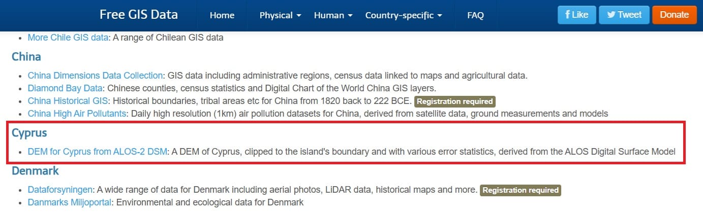
As you can see, the Digital Elevation Model (DEM) of Cyprus is available, as extracted from ALOS-2 Satellite mission [1]. But, what is the Digital Elevation Model (DEM)?

According to USGS definition, a Digital Elevation Model (DEM) is a representation of the bare ground (bare earth) topographic surface of the Earth excluding trees, buildings, and any other surface objects. Let’s see a representation made by Simou et al. (2014) [2].

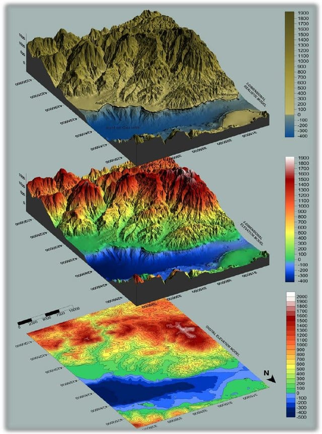
This is a Digital Elevation Model (DEM), 3D Elevation Model and 3D Realistic Model of the combined marine & land surface data, presenting the morphology of a study area. When we download the data for Cyprus, we will see a 2D representation (flat representation like the bottom image above). In the next lessons, we will also create a 3D Visualization of a Digital Elevation Model (DEM)!

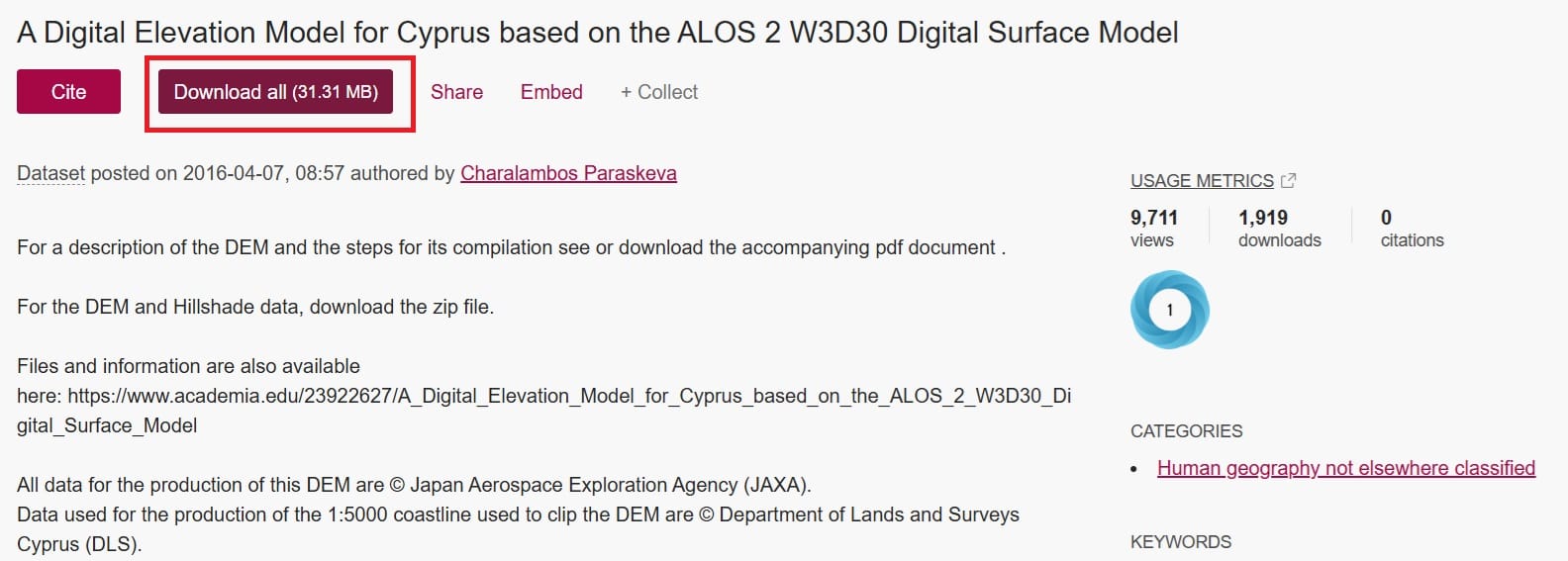
Let’s go back to the Cyprus DEM! By pressing the ‘Download’ button, we can save the DEM raster data.

Step 2: That was way too easy! Let’s find some additional raster data, for other variables, for example, the wind speeds of Cyprus.

To do that, we will visit the Global Wind Atlas website, created by the Denmark Technical University (DTU).

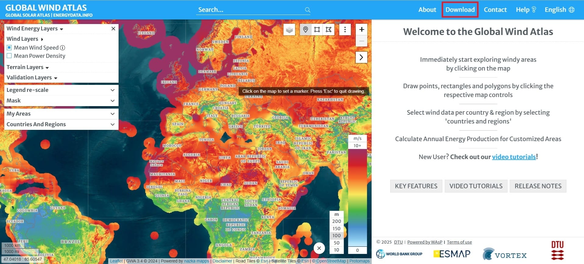
With the Global Wind Atlas webiste you can visualize and extract images on the fly for the ‘Mean Wind Speeds’ globally, the ‘Mean Power Density’ or the ‘Bathymetry’ among other variables. However, the Global Wind Atlas repository has a geospatial database where we can download and process all these data using different GIS Platforms like QGIS!

On the top right corner, if you press the ‘Download’ button and then the ‘GIS files & API access‘, you may donload all of the aforementioned raster datasets for any country wordwide.

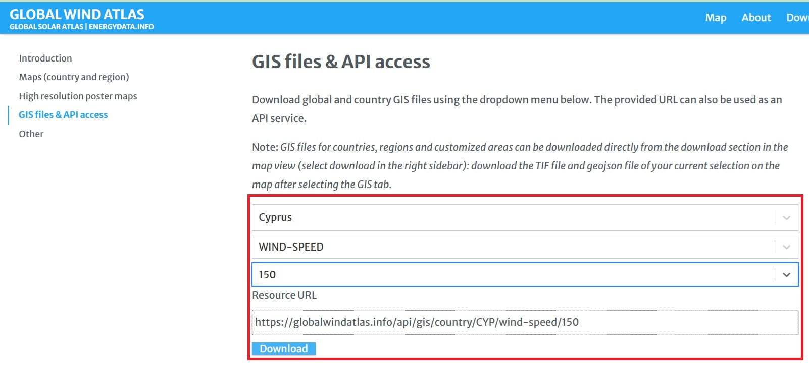
Let’s try to download the ‘WIND-SPEED’ raster file for Cyprus at a height of ‘150’ meters above sea level. Why 150 meters? Let’s imagine that we want to identify optimal areas for placing offshore wind turbines! After we select the appropriate variables, we click on the ‘Download’ button.

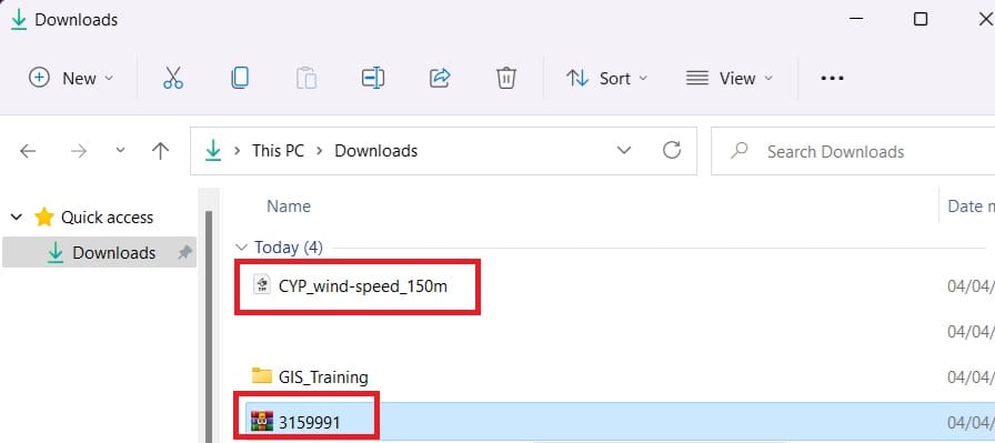
We have now downloaded both the DEM file and the wind speeds. The DEM file should be extracted (we should also extract the ‘ALOS2_Cyprus’ file inside ‘3159991’ folder). In contrast, the ‘CYP_wind-speed-150m’ is a .tiff file (the most well-known raster data type) so, we don’t have to extract any data. We copy both datasets in our ‘GIS_Training_ folder where we store the shapefile data we’ve downloaded during the previous lesson!

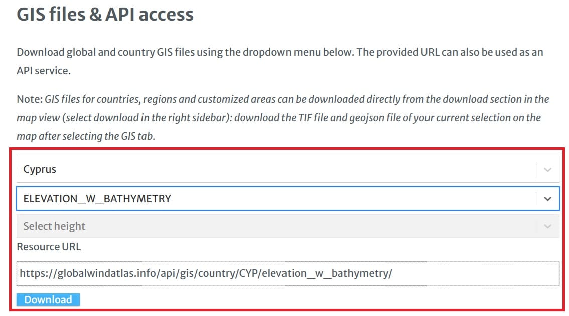
Step 3: In the same way, you can also download from ‘GIS files & API access‘ the Bathymetry of Cyprus (‘Elevation_w_Bathymetry’ raster) and copy it to your ‘GIS_Training’ folder.

Step 4: Let’s load our raster files on QGIS Platform!

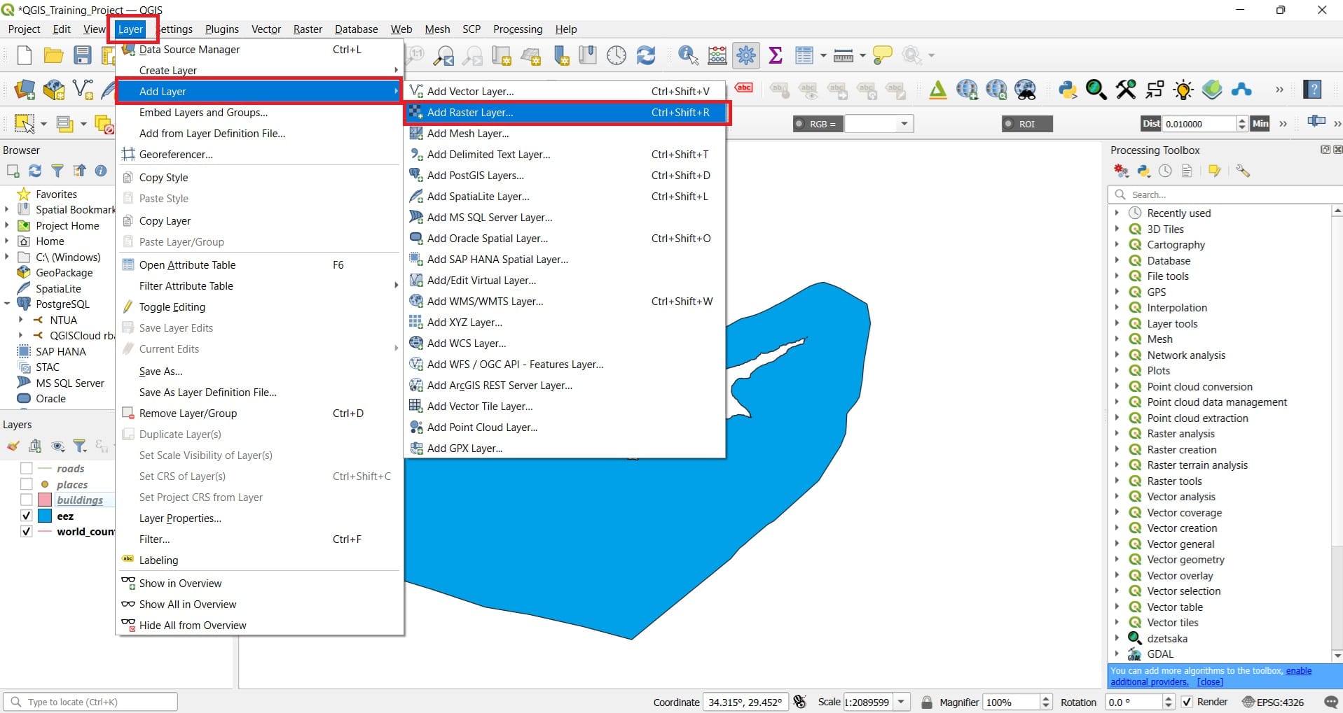
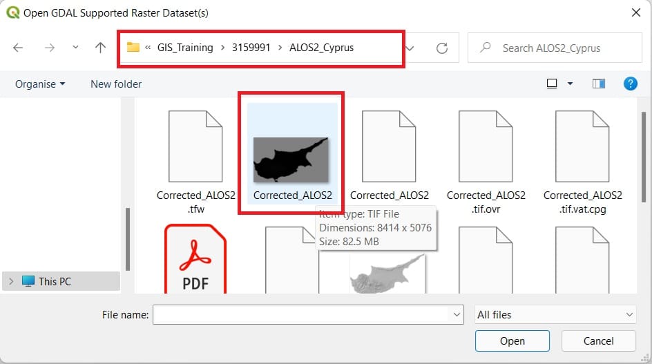
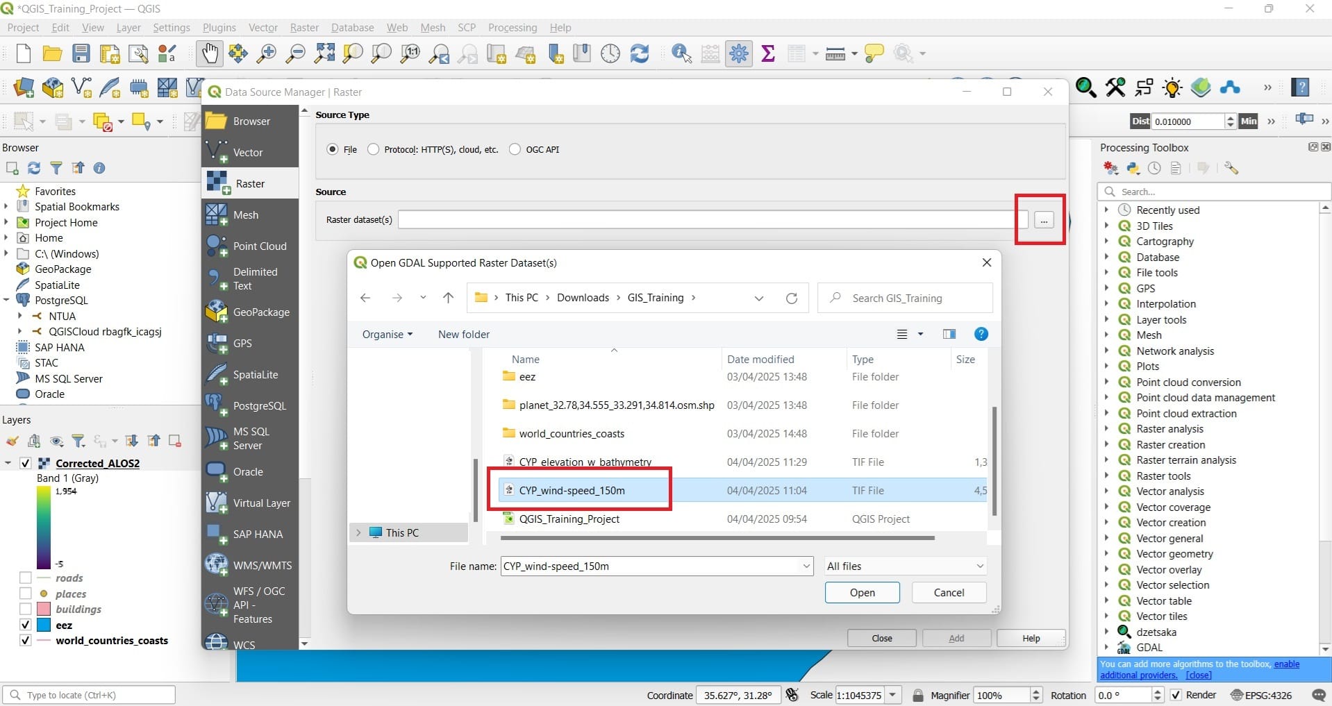
In the same way we loaded our shapefiles, we will go to the ‘Main Toolbar’ > ‘Layers’ > ‘Add Layer’ > ‘Add Raster Layer’ and then we browse in our ‘GIS_Training’ folder inside ‘3159991’ > ‘ALOS2_Cyprus’ > ‘Corrected_ALOS2’ (the .tiff file).

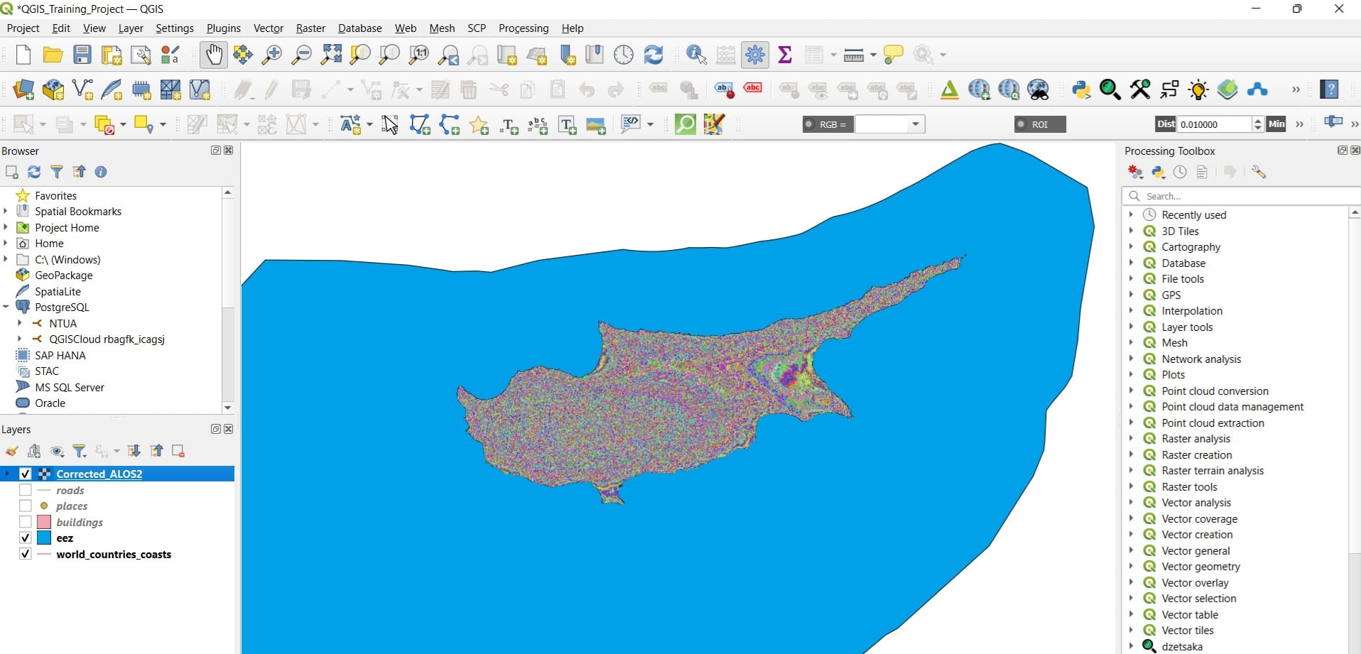
After we press ‘Open’ > ‘Add’, the results will look like this.

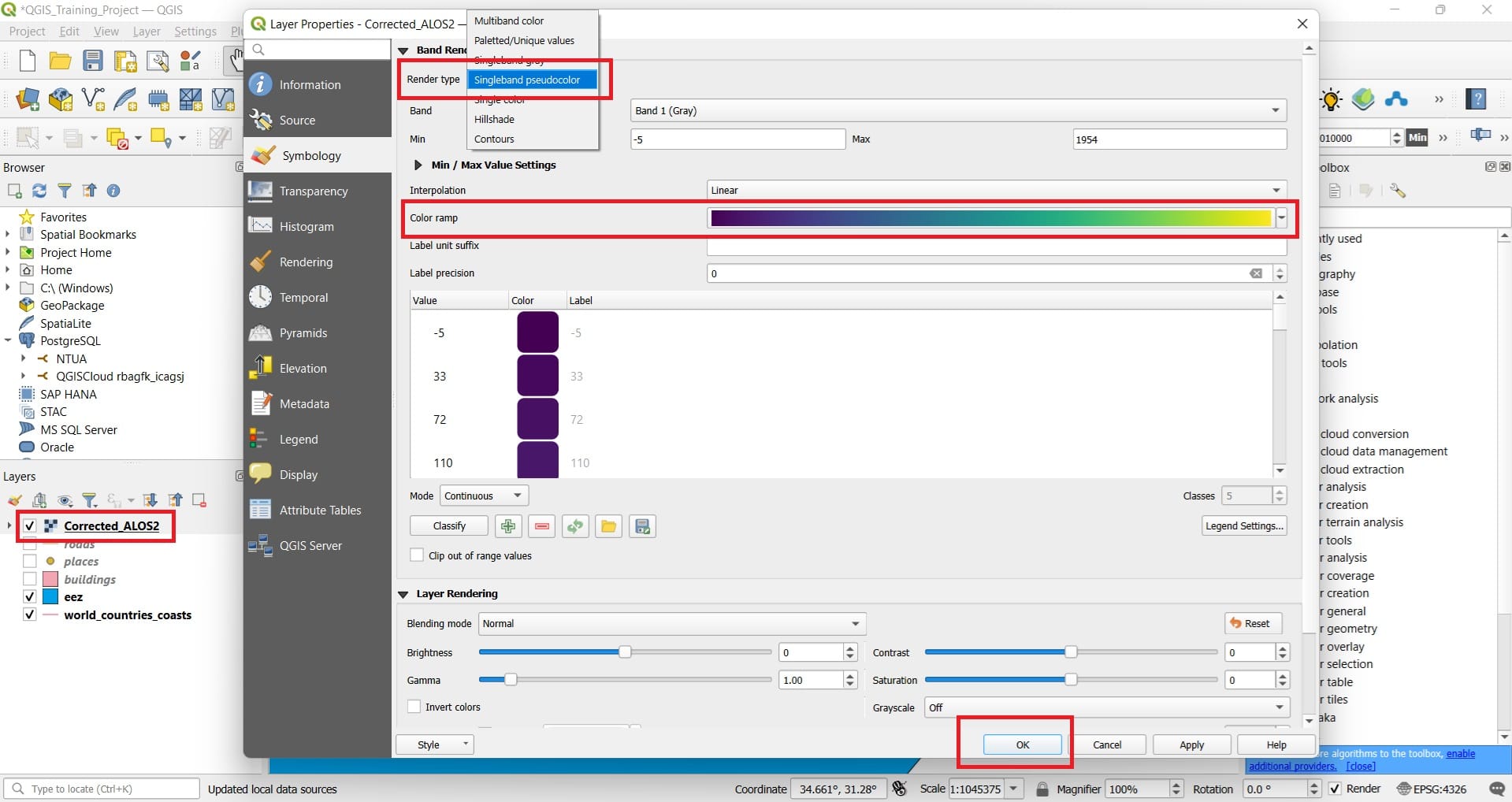
Ok, not so impressive but, we can play a little bit with the color palette! We can double-click on ‘Corrected_ALOS2’ in the ‘Layers’ tab > Symbology > ‘Render type’ > ‘Singleband pseudocolor’ > ‘Color ramp’ > Viridis > Ok.

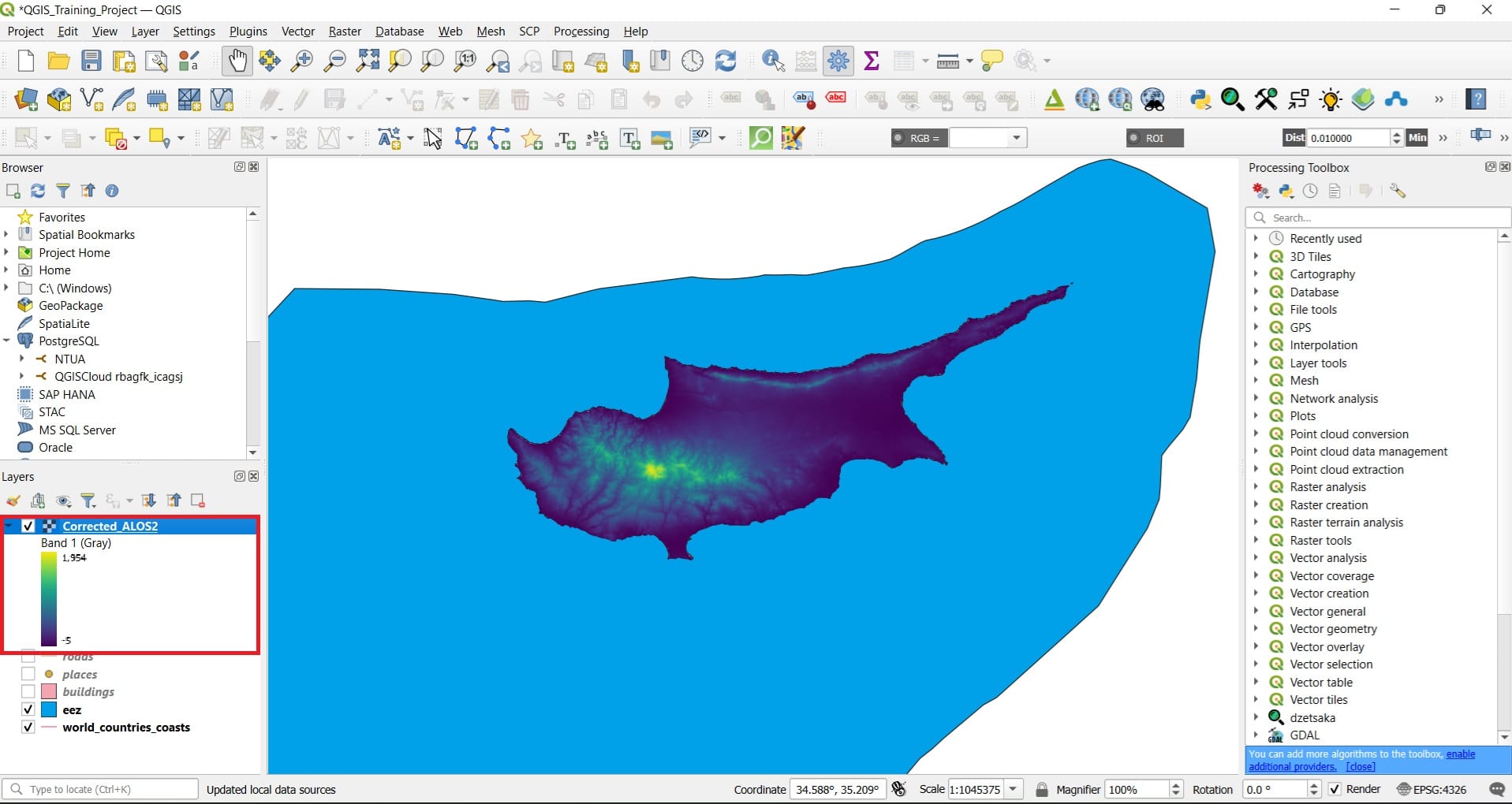
The visualization results will look more impressive and now we can easily identify where the mountaneous areas are! If we press the ‘Arrow’ button in ‘Corrected_ALOS2’ raster on the ‘Layers’ panel we may see the scale and the colours differentiations! Hence, yellow colour areas are high mountaneous areas (up to 1954 meter altitude) and the dark blue areas are flat areas!

Let’s try to load the ‘Wind_Speed_150’ raster as well! In the same way we navigate from ‘Layers’ > ‘Add Layer’ > ‘Add Raster Layer’ and browse to the ‘CYP_Wind_Speed_150’ .tiff file.

In the same way, after we load the .tiff file, we change the color palette by double-clicking on ‘CYP_Wind_Speed_150’ in the ‘Layers’ tab > Symbology > ‘Render type’ > ‘Singleband pseudocolor’ > ‘Color ramp’ > Turbo > Ok.

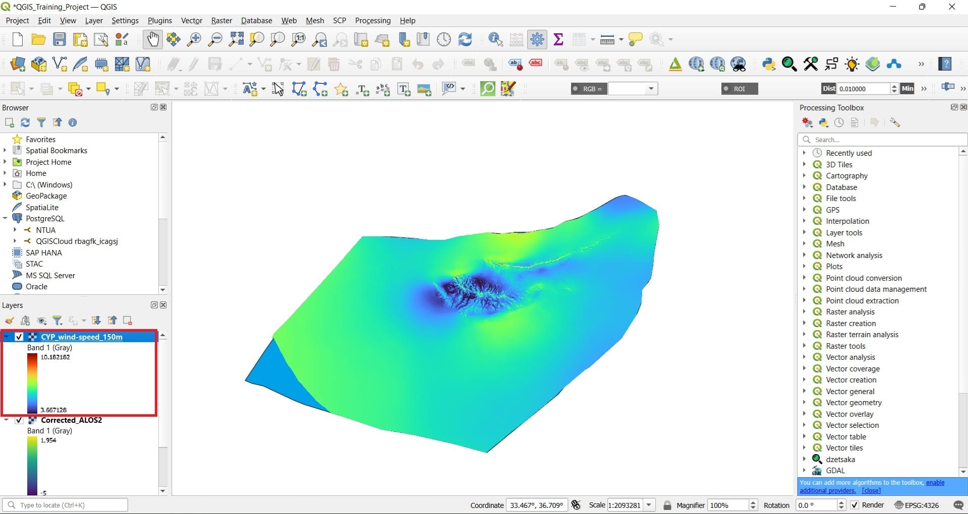
We can see that the windiest areas (red colour) are on top of the highest mountains in Cyprus, dark blue areas are not wind at all and the yellow color areas have medium wind speeds.

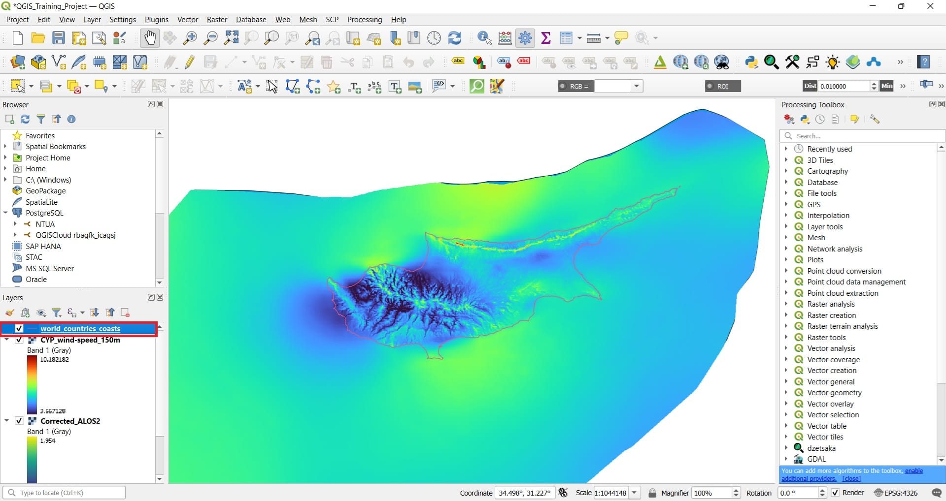
You can also drag the shoreline file (‘world_countries_coasts) on top so that you can see the Cyprus shoreline overlayed on top of the wind speed and the DEM data.

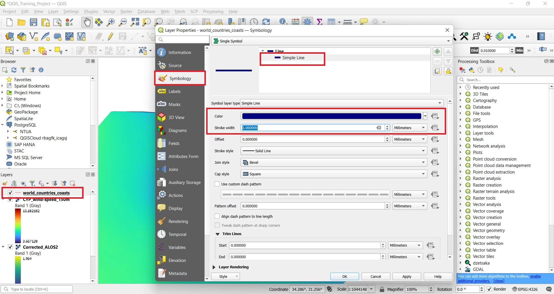
You can always change the shoreline width and color by double-clicking on the ‘world_countries_coasts’ shapefile > Symbology > Simple line > and change the ‘Color’ and the ‘Stroke width’.

And the result will look like this! DON’T FORGET TO SAVE YOUR PROJECT!

That was it! We have now loaded our first raster datasets! What is next? To find vector or raster datasets online, without downloading any data on our computer! Is that possible? Yes, fortunately!

You may also check the following videos explaining how to load raster data and change the visualization colors!

Useful links

1. ALOS-2: Satellite Mission information
2. Simou et al. (2014). Coastal hazard related to landslide distribution derived from morphotectonic analysis. Conference: 10th Int. Congress of the Hellenic Geographical SocietyAt: Thessaloniki, Greece