Creating new files and digitizing objects

Introduction 

In GIS, digitizing is the process of creating new spatial data by manually drawing features like points, lines, or polygons on a map. This is especially useful when existing data is incomplete, outdated, or when you want to map features based on your own observations or research. In QGIS, this involves creating new shapefiles and using editing tools to digitize geographic objects.

In this lesson, you’ll learn how to create your own vector layers from scratch and add new features through the digitizing process. This skill is essential for custom mapping projects, field data entry, and adding local knowledge to your GIS work.

By the end of this lesson, you will:

✅ Understand how to create new shapefiles for points, lines, or polygons in QGIS.
✅ Learn how to define and customize the attribute table for your new layers.
✅ Activate editing mode and use digitizing tools to add and modify features.
✅ Practice saving and managing your edits safely.
✅ Gain confidence in building your own spatial datasets from scratch.

Let’s get started by learning how to build your own geospatial layers in QGIS!

Digitizing new features

Now that we have successfully created a new project, let’s zoom-in a little bit more in Athens, so that we are able to identify different green infrastructure!

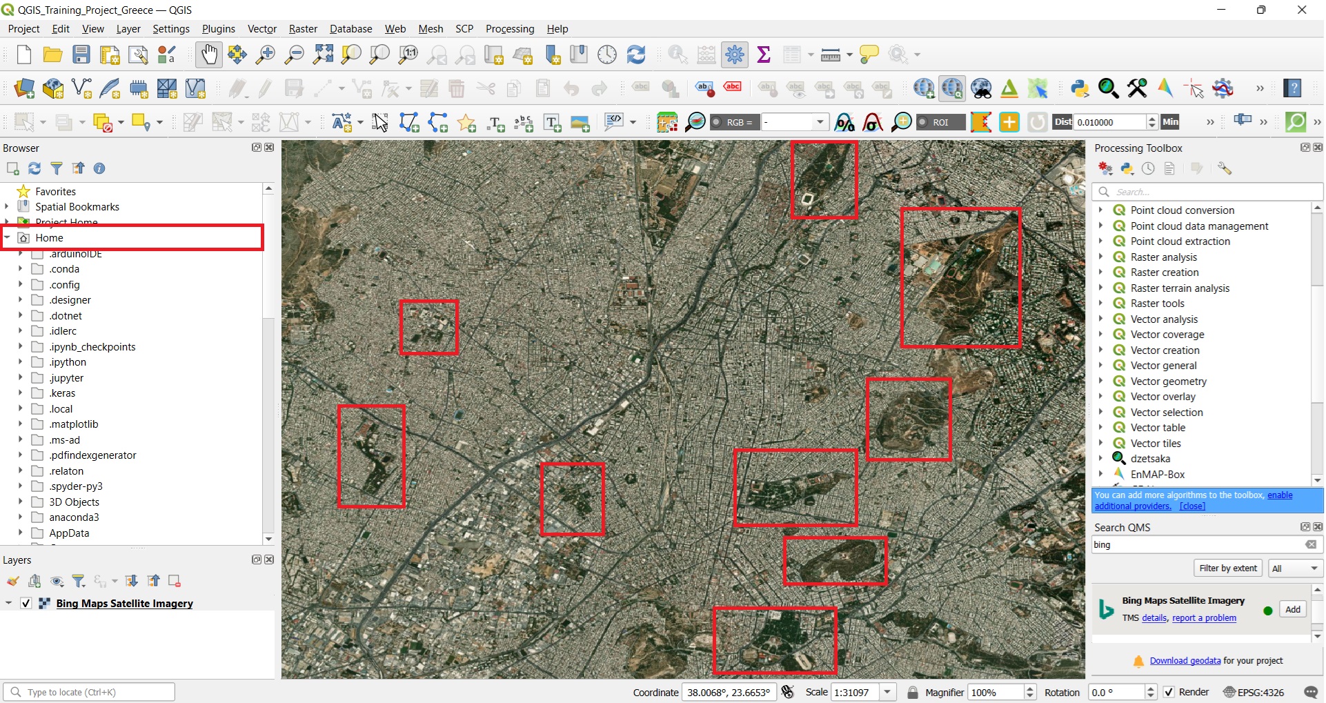
Our goal is to digitize the areas highlighted in the red boxes (see image above). To do that we have to create a new shapefile (vector dataset) in our folder. Before we create our new shapefile, let’s refresh our memory on the different vector data structures! In particular:

• Points may represent discrete locations defined by a single coordinate pair (X, Y). They are ideal for features too small to be depicted as lines or areas, such as individual trees or lamp posts.
• Lines (or polylines) are sequences of points connected to represent linear features like roads, rivers, or pipelines.
• Polygons are closed shapes formed by connecting multiple lines, used to represent areas such as parks, lakes, or city boundaries.

Scale and Representation: The choice between points, lines, and polygons often depends on the map’s scale:

• At a large scale (zoomed in), features like the green areas of Athens are best represented as polygons, allowing for detailed digitization of their boundaries.
• At a small scale (zoomed out), the same green areas might appear as small spots, making points a more appropriate representation due to the reduced detail.

Understanding these vector data structures and their relationship with scale is crucial for accurate and effective GIS mapping and analysis. In our example, we are considering that the green areas of Athens can be digitized and represented as polygons.

To create a new shapefile, we may use either the ‘Browser’ window (red box on the image below) or the ‘Layer’ tab on the QGIS main toolbar (green box) > ‘Create Layer’ > ‘New Shapefile Layer’.

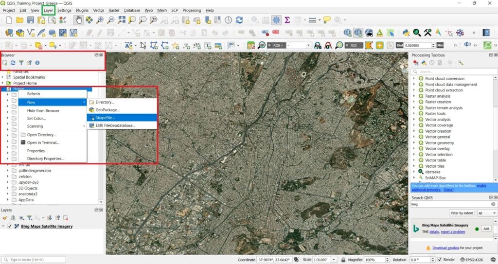
With both options options, we should browse and select the folder we want to create our new shapefile. Let’s try to create our new shapefile in the ‘GIS_Training’ folder. You may create a new sub-folder ‘Greece’ and save your new shapefile.

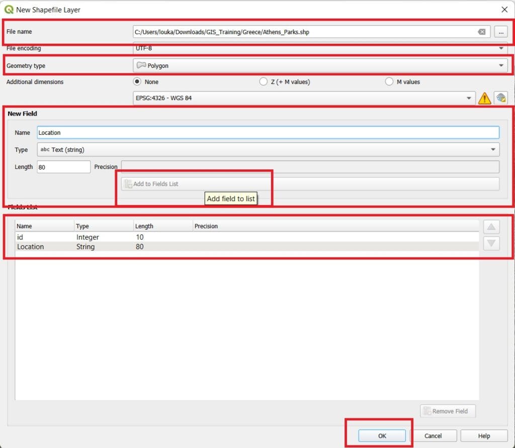
First, we must select a ‘proper’ name for our new shapefile. ‘Athens_Parks’ is quite descriptive and clear but, feel free to name your shapefile as you wish! Then, we must select the geometry type (i.e. point, line, polygon) and as we mentioned, our new shapefile has a ‘polygon’ geometry type.

Do you see the field ‘EPSG:4326 – WGS 84’? If you remember from the previous lessons, that’s the Coordinate Reference System (CRS)! It’s a geographic one and we will keep it as it is for now. Why? Because all basemaps, like the ‘Bing Maps Satellite’ we have loaded here use WGS 84 s well! Thus, no transformations are needed to overlay new data.

In the ‘Fields List’ window, we may select to add a new field in our shapefile. In GIS, every vector layer—such as a shapefile—has an associated Attribute Table. This table stores information about each spatial feature in the layer (i.e. each polygon). Each row corresponds to a feature (like a point, line, or polygon), and each column represents a specific attribute or field describing that feature. For example, since we’re digitizing green areas in Athens, each polygon could have attributes like its name, area, or type of vegetation. We will create a new field named ‘Location’ in order to add the areas that each park is located.

Then we press ‘Add to Fields List’ and our new field has been added. To create our new shapefile we press ‘OK’ and then we load (drag and drop, red box on the image below) our new ‘Layer’ on QGIS main toolbar (green box on the image below) > ‘Add Shapefile Layer’ > Browse to your folder.

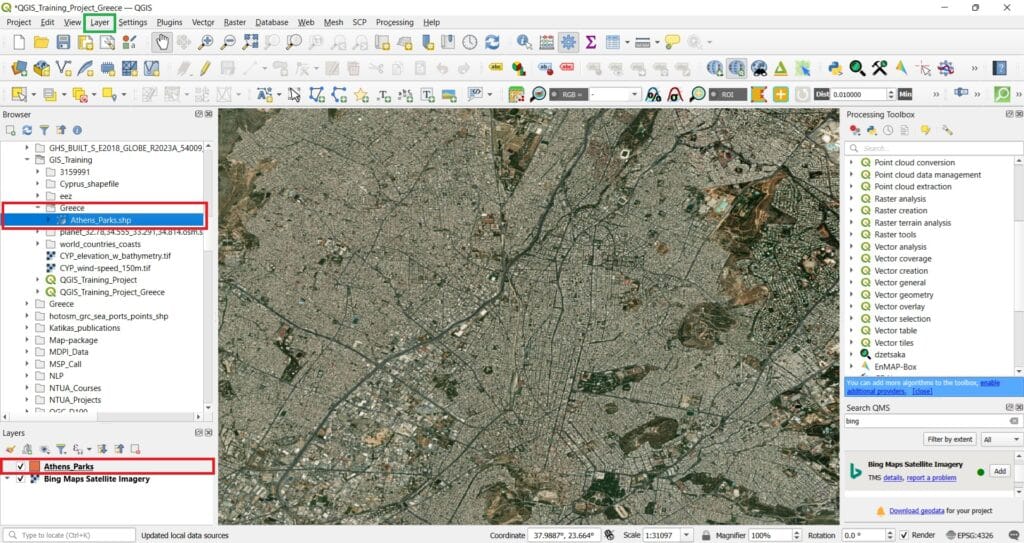
After we load our new shapefile, we don’t see any change! Why? Because it is empty. Let’s start then adding information and digitizing green areas!

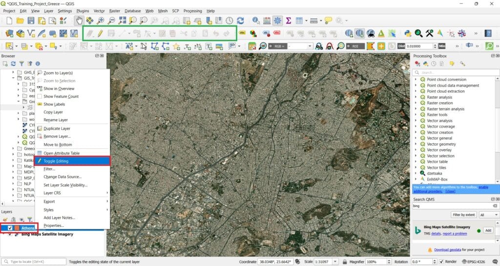
To do that, we just right-click on our shapefile ‘Athens_Parks’ > we press ‘Toggle Editing’, which means activate/enable editing! After we activate editing, the ‘Toggle Editing’ bar will be activated (green box on the image below) and in particular, the ‘Add Polygon’ icon (the icon with the green polygon).

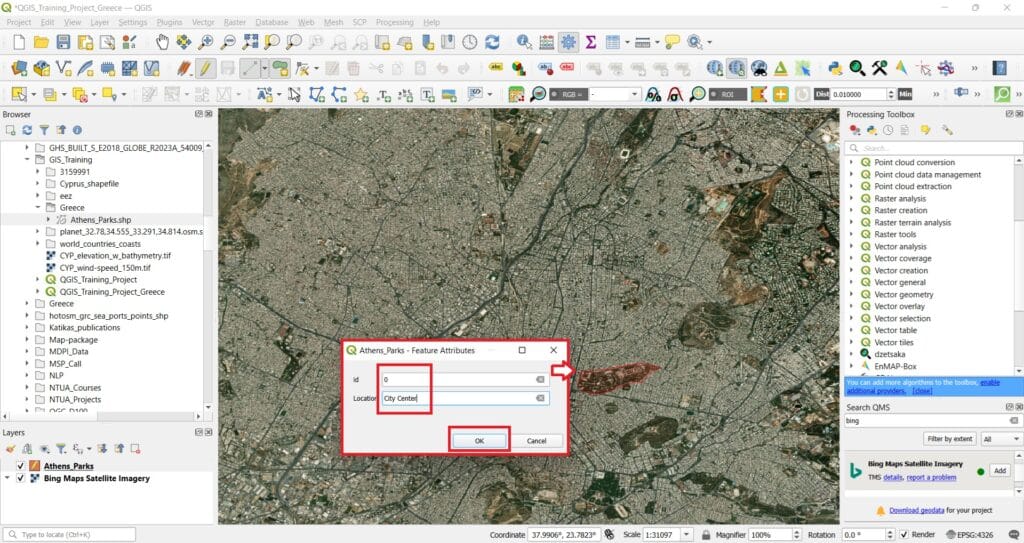
After we select the ‘Add Polygon Feature’ icon, we can start the editing process! Let’s digitize the polygon near the city center (refer to the image below). To begin editing, left-click with your mouse to add points along the polygon’s perimeter until the entire area is covered.​ This process involves creating a new polygon feature by sequentially placing vertices that define the shape’s boundaries. Once all vertices are placed, right-click to finalize the polygon. Afterward, you can enter attribute information for the digitized feature.

After we add our last point, we right-click to ‘close’ our polygon and add the metadata (i.e. ‘id’ and ‘location’, see image below). Overall, in GIS and programming world, when we start counting different entities, we don’t start from 1 but from 0 (for programming purposes). Hence, our first polygon will get the ‘id’ = 0 and of course, the ‘Location’. Let’s say that the green area is located in the city center. Finally, we press ‘OK’

Let’s digitize a couple more polygons! Don’t forget to give an increasing ‘id’ to every polygon you are digitizing, for example, polygon 1 (id = 0), polygon 2 (id = 1) etc. Also, add the location information every time you finish a polygon (right-click). Let’s give a location name of ‘Lycabettus’ for our second polygon (below our first polygon) and ‘Galatsi’ for our third polygon (the big one on the top right corner).

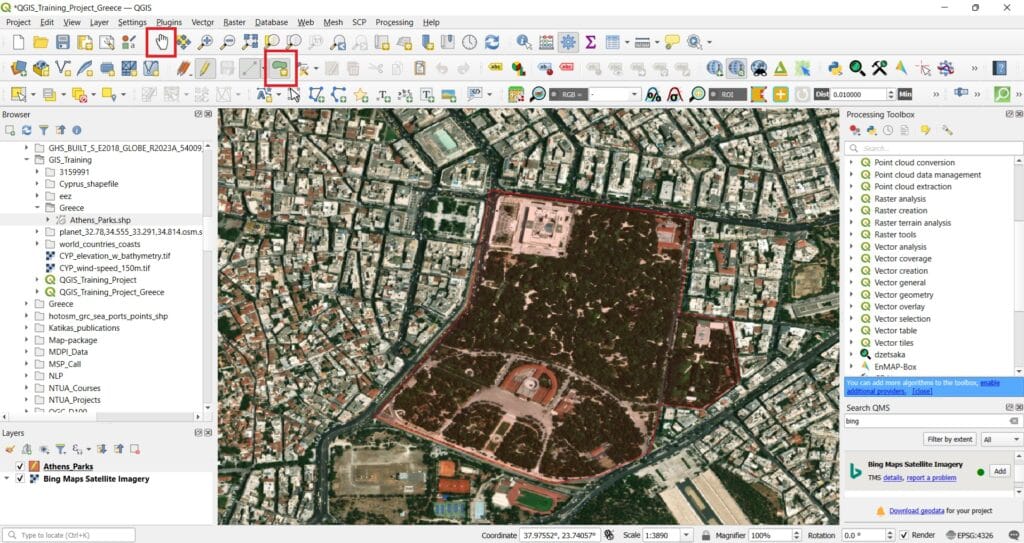
Of course, if you want to be more precise during the digitization process, feel free to zoom-in for more detailed editing (see the image below)! You can always the ‘Pan Map’ icon to move your basemap or any Layer you want in order to find a specific area and then, by clicking again the ‘Add Polygon’ button you can keep editing the area you want!

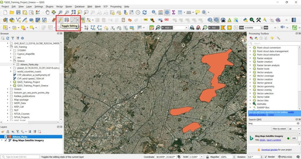
After we finish the digitization process, we press ‘Toggle Editing’ (see image below) and > ‘Save edits’. That was it! We’ve create our first spatial dataset!

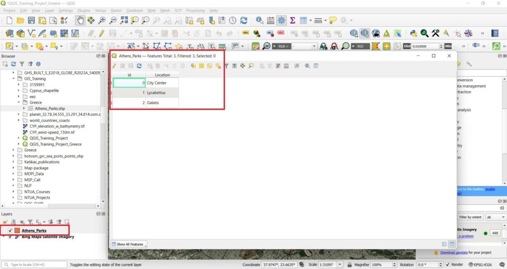
If we right-click on the ‘Athens_Parks’ shapefile we’ve created and then select > ‘Open Attribute Table’, we should see something similar to the image below. Three different polygons have been created with 2 different attributes each, an ‘id’ (unique id) and the ‘Location’!

For more instructions on how to digitize data, check out the following video!

Reprojecting Layers

In QGIS, reprojecting vector and raster layers is essential for ensuring spatial accuracy and consistency across your GIS projects. While QGIS offers “on-the-fly” CRS transformation as we mentioned in the previous lessons, which allows layers with different Coordinate Reference Systems (CRS) to be displayed together seamlessly, there are compelling reasons to perform permanent reprojection of your data layers [1].

Why Reproject Layers in QGIS?

1. Ensure Spatial Alignment: Reprojecting layers to a common CRS ensures that all spatial data aligns correctly. This is crucial when overlaying multiple datasets, as mismatched CRSs can lead to misaligned features and inaccurate analyses.
2. Improve Performance: While “on-the-fly” reprojection is convenient, it can introduce computational overhead, especially with large or complex datasets. Permanently reprojecting layers can enhance performance and reduce processing time during analysis.
3. Accurate Spatial Analysis: Certain spatial analyses, such as distance and area calculations, require data to be in a projected CRS that preserves these measurements. Using an appropriate projected CRS ensures the accuracy of your analytical results.
4. Data Integrity: Reprojecting layers allows you to maintain the integrity of your data by ensuring that all layers share the same spatial reference. This is particularly important when sharing data with others or integrating datasets from various sources.

How to Reproject Layers in QGIS:

• Vector Layers: Right-click on the vector layer in the Layers panel, select “Export” > “Save Features As…”, and choose the desired CRS in the dialog that appears.
• Raster Layers: Use the “Warp (Reproject)” tool found under “Raster” > “Projections” > “Warp (Reproject)” in the Processing Toolbox.

Let’s put it into practice with our previous example and the new polygon shapefile we have created! Remember, the Coordinate Reference System (CRS) of the shapefile we’ve created was WGS 84 (geogrpahic CRS)!

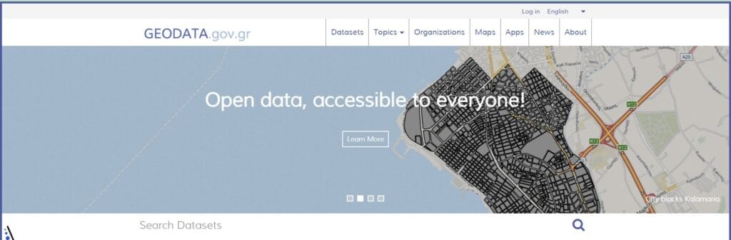
Let’s download some additional data for Athens! To do that, we will use the national geoportal with different types of geospatial data (http://www.geodata.gov.gr/en/).

Using the following links, we will download one additional dataset (vector data as shapefile) for Athens. In particular, the boundaries (as polygons) of different districts of the Municipality of Athens.

Shapefile data link: http://www.geodata.gov.gr/en/dataset/op1a-re1tov1wv-anuou-a0nvaiwv

Of course, you may download any kind of spatial data from the geodata portal by selecting ‘Datasets’. By clicking the link above, you will see the following image!

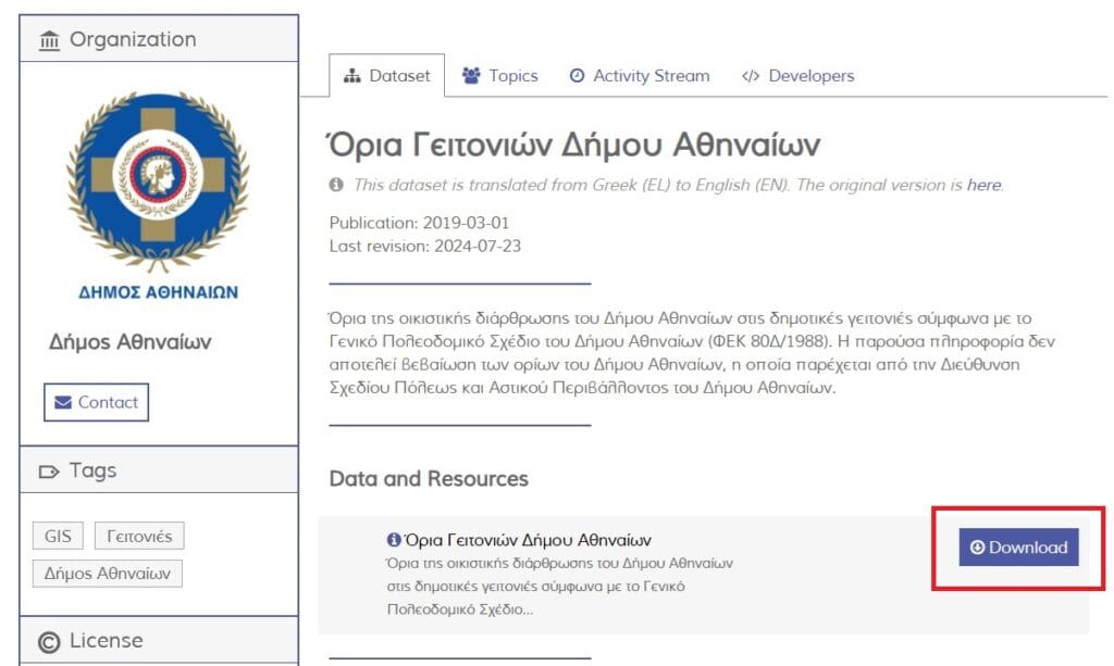
If you press ‘Download’, a zipped file will be downloaded. Cut and paste the zipped folder in the ‘GIS_Training’ data folder > ‘Greece’ sub-folder. Then extract the data. The name of the shapefile is ‘geitonies’, which means ‘neighborhoods’. But why is everything in Greek? Probably because this dataset is mainly used by users in Greece however, we should be a bit more suspicious! Since everything is in Greek, maybe the coordinate system (CRS) of this shapefile is a Greek one!

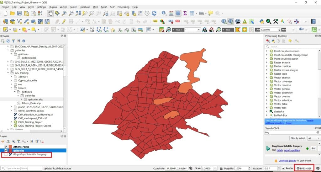
That’s correct! It’s the ‘Greek Grid (EPSG:2100)’! How do we know that? Let’s load the new dataset on QGIS.

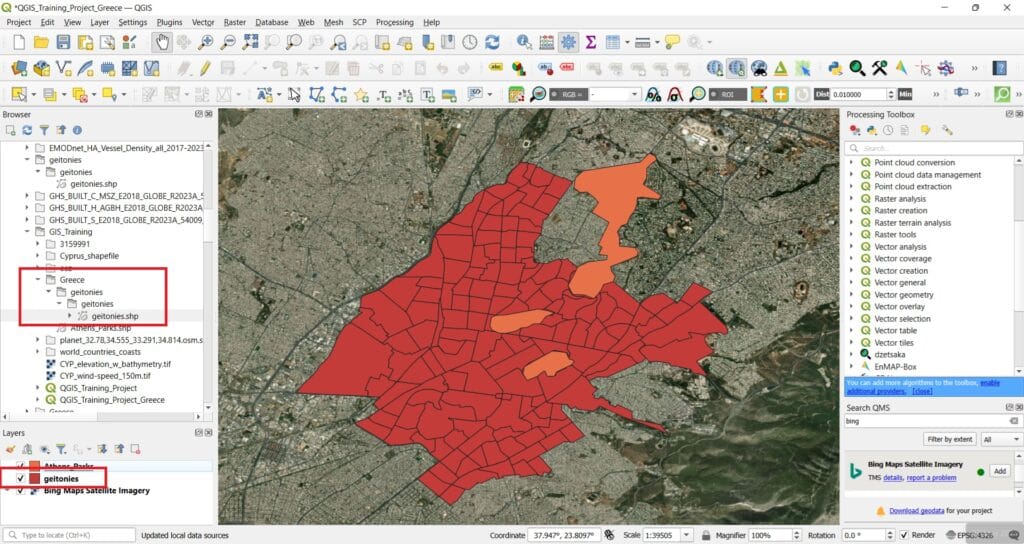
Do you see anything unusual? Probably not. As it seems, the new dataset was loaded properly even if the CRS is different. How do we know that? Let’s double-click the ‘geitonies’ shapefile in the ‘Layers’ window.

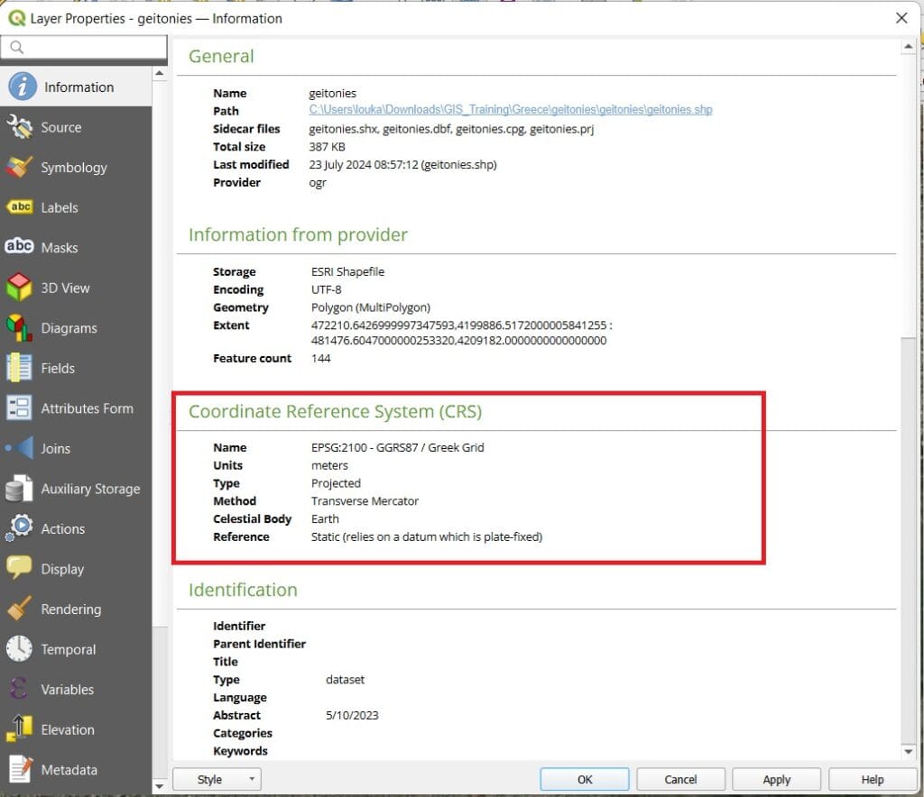
If we check the ‘Information’ tab (see the image above), the CRS of the dataset is the ‘Greek Grid’ however, the CRS of the ‘Athens_Parks’ we have have created, is the WGS 84. Don’t forget ‘On the fly’ CRS transformation that GIS platforms apply when loading spatial data with different CRS.

If we want to see the actual distortion caused by loading spatial datasets with different CRSs, let’s try the following exercise! We can hide the ‘Bing Maps Satellite’ and then on the bottom right corner of QGIS interface we can double-click on the ‘EPSG:4326’ button. In this way, we may change the CRS of our project in QGIS.

When we double-click on ‘EPSG:4326’ a new window appears! It’s the same window if we alernatively select ‘Project’ on the main QGIS toolbar > ‘Properties’ > ‘CRS’. On the new window, we check the button ‘No CRS (unkown CRS…)’ > we press ok. Something disappeared right?

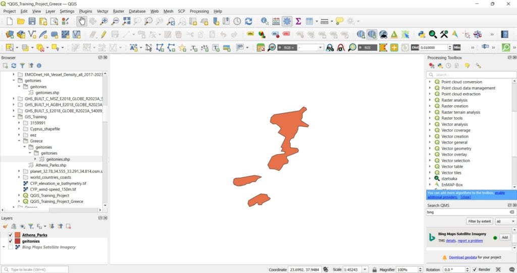
The ‘geitonies’ shapefile suddenly disappeared. Actually, it didn’t disappear, it was moved somewhere far far away since the initial dataset we created had a geographic CRS (WGS 84) using φ and λ (in degrees) as coordinates and the new shapefile we’ve loaded uses a projected CRS with x and y as coordinates (in meters). The numbers for WGS 84 are in decimal degrees format and range from -90 to 90 for latitude and -180 to 180 for longitude. This means that QGIS platform understands that the ‘geitonies’ shapefile has also a geographic CRS and sent it far far away where the x and y values in meters are located (considering that it’s φ,λ). Which are the actual coordinates of the ‘geitonies’ shapefile extext? Approximately, x = 47000 and y = 42000 METERS not degress. That’s why we can’t see the second shapefile.

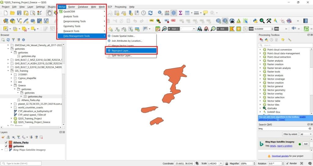
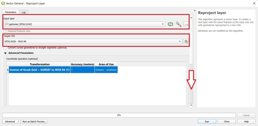
To put everything ‘back on track’ we can reproject (change CRS) one of our shapefiles! Let’s try to reproject the ‘geitonies’ shapefile. To do that, we navigate to the ‘Vector’ tab on the main toolbar > ‘Data Management Tools’ > ‘Reproject Layer’.

The ‘Reproject’ tool window will appear and then we select as ‘Input Layer’ > ‘geitonies’, ‘Targeted CRS’ > ‘EPSG:4326, WGS 84’ and if we scroll down we select to save the ‘Reprojected’ layer in the ‘GIS_Training’ > ‘Greece’ folder. You may name the new shapefile as ‘Neighborhoods_Reproject_WGS’ so that you know what exactly this shapefile is all about!

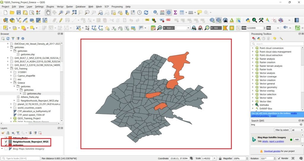
After you press ‘Run’, the shapefile will appear on the correct position it was before (see the image below). Why? Because we changed the CRS to WGS 84!

However, if you try to activate the ‘Bing Maps Satellite’ basemap, nothing changes. Why? If you remember, our current QGIS has no CRS defined! Let’s double-click on the Project CRS (bottom right corner icon with the X sign) > uncheck the ‘Unkown CRS’ button and select WGS 84 > Press ‘OK’.

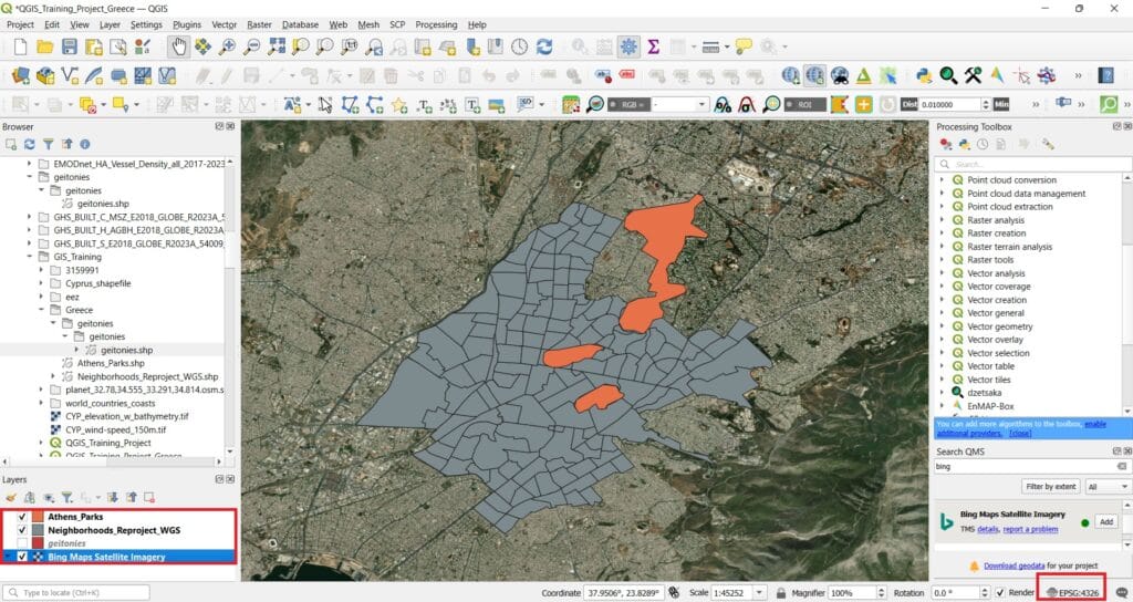
That was it! Everything looks normal again! In case you are interested on how to reproject both vector and raster data check the following videos!

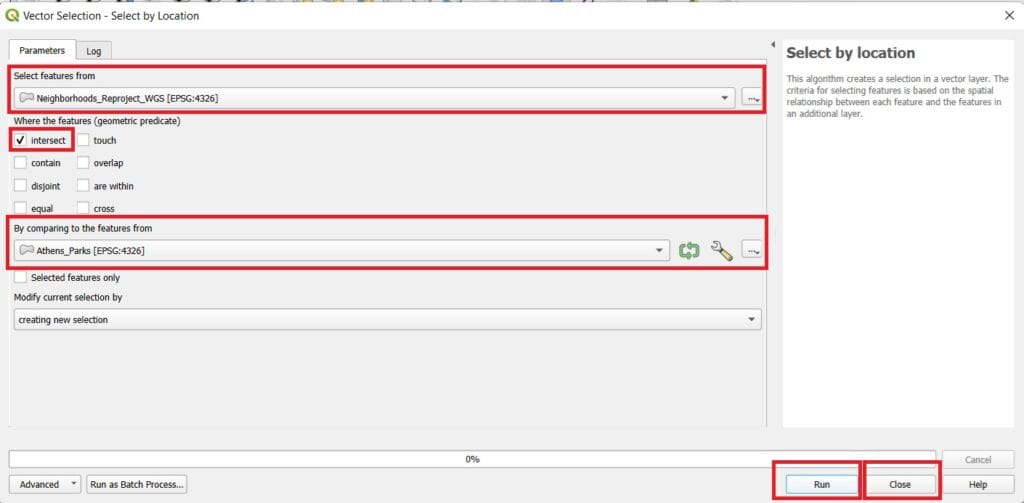
Since both of our vector datasets have the same CRS we can perform some simple spatial queries! Let’s see an example. If we select ‘Vector’ on the main QGIS toolbar > ‘Research Tools’ > ‘Select by Location’, we may start answering some ‘spatial’ queries. For example:

• The green areas we digitized, how many neighborhoods are they intersecting/crossing?

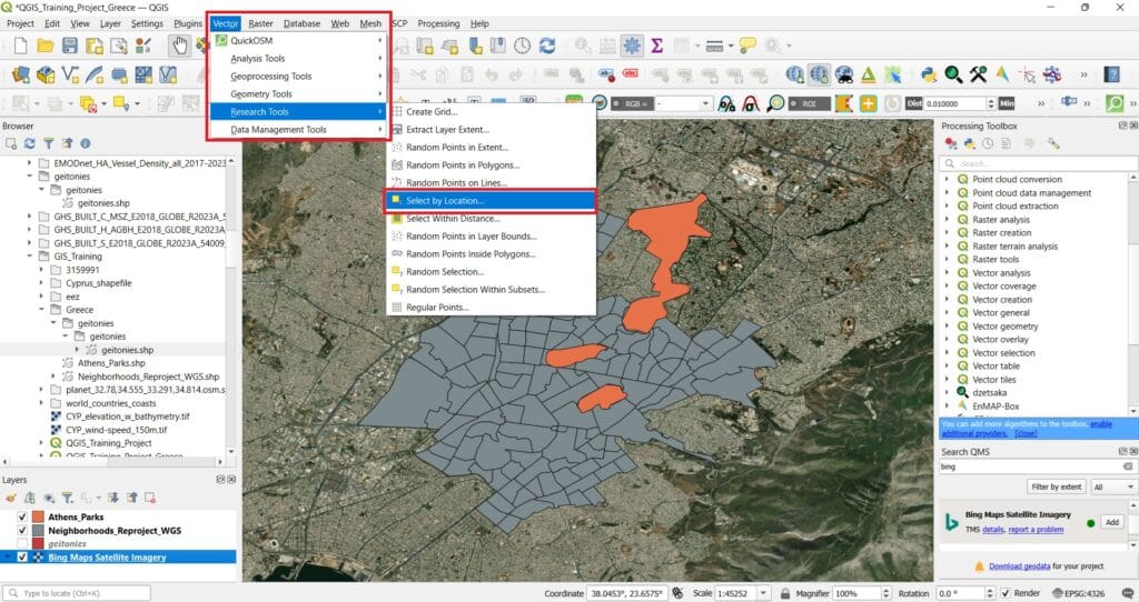
A new window will pop-up and we select ‘Select features from’ = ‘Neighborhoods_Reproject_WGS’, ‘Where the features’ = ‘intersect’, ‘By comparing to the features from’ = ‘Athens_Parks’. We press ‘Run’ and ‘Close.

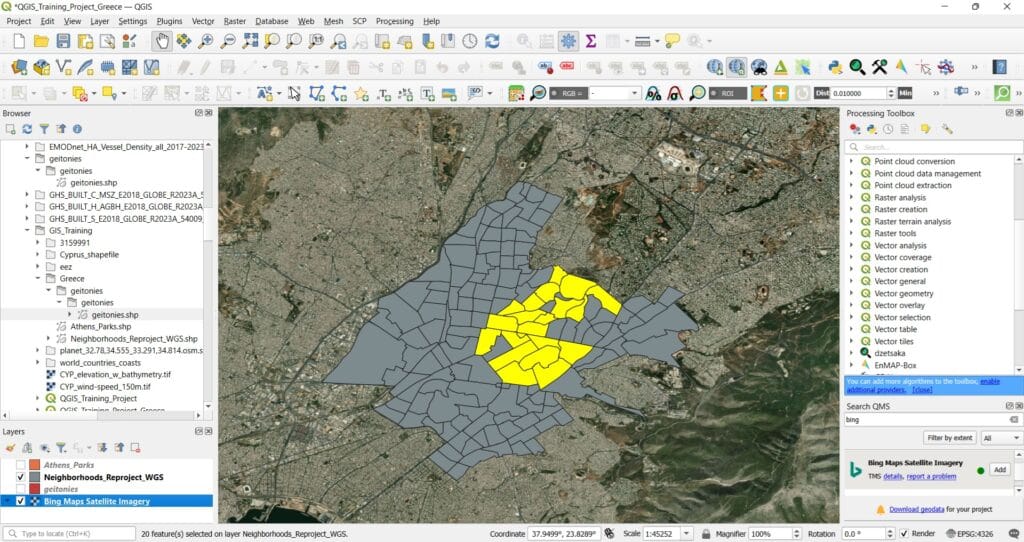
The result will look like the image below! All yellow polygons are the selected ones! Hence, the ones that are intersected with the green areas!

We can also see the attributes, for example, the names of the neighborhoods that are intersected by the green areas! If we right-click on the ‘Neighborhoods_Reproject_WGS’ shapefile > Open the Attribute Table’ > Click on ‘Show all features’ on the bottom left corner of the Attribute Table window and select > ‘Show Selected Features’

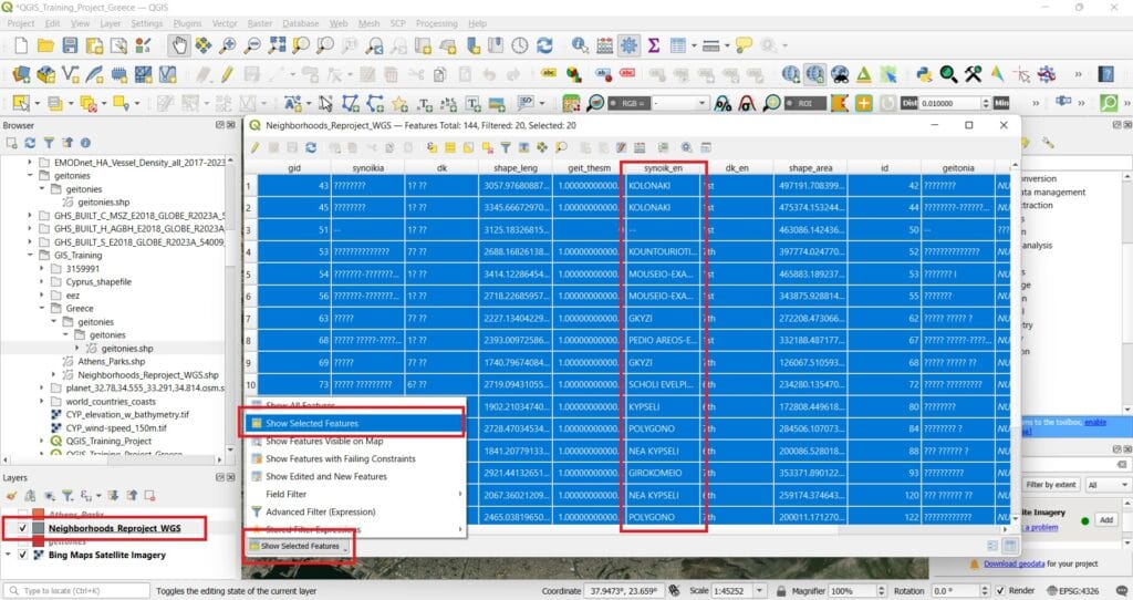
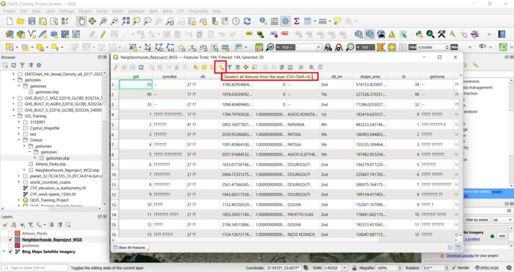
We can now see only the intersected polygons and the names of the neighborhoods, for example, ‘POLYGONO’, ‘NEA KYPSELI’ etc. In case you want to clear/de-activate the selected polygons, you can press the ‘Clear Selection’ button (see the image below) and perform a new query.

This brings us to the end of our lesson on how to create new spatial files and reproject vector and raster layers in QGIS. You’ve learned how to build your own shapefiles, digitize features, and ensure that all your data layers align correctly by working within the appropriate coordinate reference system. These foundational skills are essential for any GIS project, helping ensure accuracy, consistency, and reliable analysis.

Ok, we didn’t perform any analysis yet but, during the next lessons we will dive into the GIS analysis world!

✅ Wrapping Up: Creating New Files and Digitizing Objects in QGIS

You’ve now completed the lesson on Creating New Files and Digitizing Objects in QGIS, where you learned how to build your own geospatial datasets from scratch. Digitizing is a powerful skill that gives you full control over the data you create—allowing you to map features based on your observations, fieldwork, or local knowledge.

Throughout this lesson, you explored how to:

✅ Create new shapefiles for points, lines, and polygons
✅ Set up and customize attribute tables to store relevant information
✅ Use the editing and digitizing tools to draw and modify features
✅ Safely save and manage your edits, building clean, accurate data

Digitizing is essential not only for custom mapping and project-based learning, but also for encouraging students to interact actively with spatial data. Whether you’re digitizing school zones, local green spaces, or data from a classroom survey, you’re now equipped to create GIS layers tailored to your needs. In the next course, we’ll explore how to import and map point data from Excel files—a useful workflow for bringing external data (like field survey results or statistical tables) into your GIS project.

Well done—your maps are about to come to life with real-world data! 📍🗺️✏️