Raster processing – Surface analysis

🌄 Introduction to Surface Analysis in QGIS

In this lesson, we’ll explore the fundamentals of Surface Analysis using QGIS, focusing on key terrain attributes such as Slope, Aspect, and other derived variables. These analyses are essential for understanding the physical characteristics of the landscape, which can inform various applications like environmental planning, infrastructure development, and hazard assessment.

✅ What You’ll Learn:

• Understand Digital Elevation Models (DEMs): Learn how DEMs represent terrain surfaces and serve as the foundation for surface analysis.
• Calculate Slope: Determine the steepness or inclination of the terrain, which is crucial for assessing erosion risk, construction feasibility, and more.
• Determine Aspect: Identify the compass direction of slopes, influencing factors like sunlight exposure and vegetation patterns.
• Generate Hillshade Maps: Create shaded relief maps to visualize terrain features effectively.
• Perform Terrain-Based Queries: Use QGIS tools to extract specific terrain information, such as identifying areas with gentle slopes or north-facing aspects.

🧭 Why Surface Analysis Matters

Surface analysis provides insights into the topography of an area, which is vital for:

• Urban and Regional Planning: Informing decisions on building locations, road networks, and zoning.
• Environmental Management: Assessing habitats, watershed boundaries, and potential erosion zones.
• Disaster Risk Reduction: Identifying areas susceptible to landslides, floods, or other hazards.

In our previous lessons, we’ve worked with Digital Elevation Models (DEMs) to analyze terrain and derive meaningful insights. Now, let’s delve deeper into what DEMs are, how they’re created, and why they’re indispensable in spatial analysis.

What Is a Digital Elevation Model (DEM)?

A Digital Elevation Model (DEM) is a digital representation of the Earth’s surface topography. It captures elevation data in a gridded format, where each cell (or pixel) holds a value corresponding to the terrain’s height at that location (without including building, trees or any other objects). DEMs provide a foundational dataset for various geospatial analyses, enabling us to model and visualize the Earth’s surface in three dimensions. In contrast, a Digital Surface Model (DSM) is a representation of the earth’s surface, including all objects, for example, trees and buildings. [1, 2].

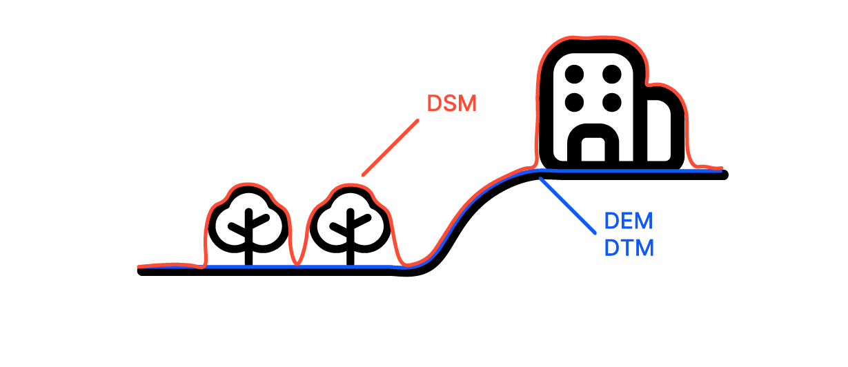
Image source: Atlas, https://atlas.co/blog/comparing-dem-dsm-and-dtm/

You may also check the following video explaining the differences!

How Are DEMs Created?

DEMs are generated using several Remote Sensing and Surveying techniques [3]:

• LiDAR (Light Detection and Ranging): Employs laser pulses emitted from airborne sensors to measure distances to the Earth’s surface, producing highly accurate elevation data.
• Photogrammetry: Involves extracting elevation information from overlapping aerial or satellite images through stereoscopic analysis.
• Radar Systems: Utilize radar signals from satellites to capture elevation data, effective even in cloud-covered regions.

These methods result in DEMs with varying resolutions and accuracies, suitable for different applications. DEMs are integral to numerous fields due to their versatility and they are used as a primary source of spatial information in:

• Hydrology: Modeling water flow, delineating watersheds, and predicting flood zones.
• Urban Planning: Assessing terrain suitability for infrastructure development and analyzing slope stability.
• Environmental Management: Monitoring erosion, land degradation, and habitat suitability.
• Disaster Risk Assessment: Identifying areas prone to landslides, floods, and other natural hazards.
• Agriculture: Planning irrigation systems and managing land based on terrain characteristics.

Importance of DEMs in GIS

In GIS, DEMs serve as a critical input for various geospatial analyses:

• Slope and Aspect Calculation: Determining the steepness and orientation of terrain surfaces.
• Hillshade Generation: Creating shaded relief maps to visualize terrain features effectively.
• Viewshed Analysis: Identifying visible areas from a specific point, useful in telecommunications and surveillance planning.
• Contour Mapping: Producing contour lines that represent elevation changes, aiding in topographic mapping.

By leveraging DEMs in QGIS for example, we can perform detailed terrain analyses that inform decision-making across various disciplines. Let’s try it out!

As you can see from FreeGIS data, there are many different platforms and repositories available for downloading Digital Elevation Model (DEM) data. These include global datasets, national portals, and open data repositories that offer elevation information in various formats and resolutions.

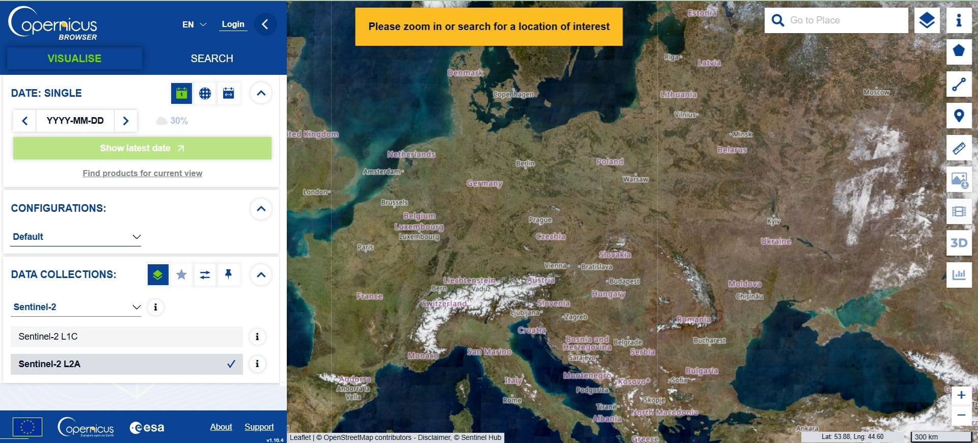
However, one of the easiest and most user-friendly ways to access global DEM data is through the Copernicus Open Access Hub (often referred to as the Copernicus Browser). This platform provides high-resolution satellite imagery and raster data, including elevation models, freely accessible to users across the world.

📝 Steps to Access DEM Data via the Copernicus Browser:

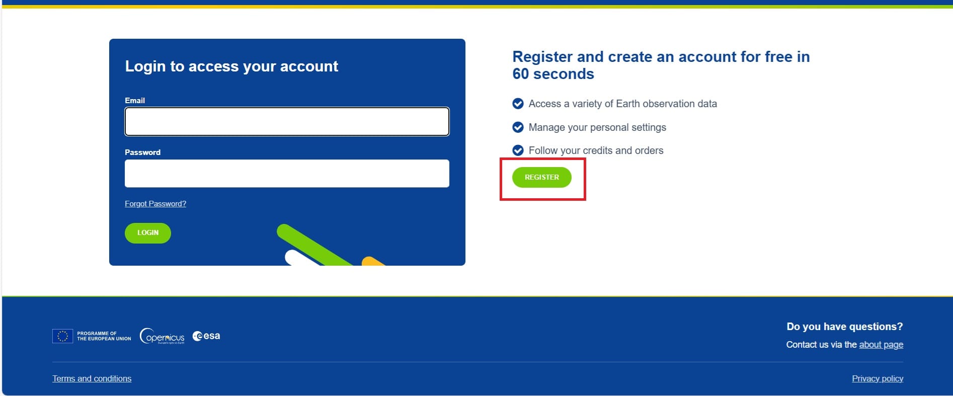
1. Register for an account – Registration is free and gives you access to download data. Just click on the ‘Login’ button and then ‘Register’ (see the image below)
2. Browse the map interface – You can select your area of interest directly on the world map.
3. Choose your data type – For elevation data, select the appropriate satellite product (such as Sentinel-1 or Sentinel-2).
4. Download in multiple formats – You can download images in formats like .jpeg for quick viewing or .tiff (GeoTIFF) for use in GIS software like QGIS.

✅ This method is reliable, regularly updated, and ideal for educational and research purposes.
✅ The .tiff files are raster images that contain georeferenced elevation values—perfect for terrain analysis, slope calculations, and 3D surface modeling in QGIS.

Whether you’re conducting a school-based GIS project or building a real-world analysis, the Copernicus Browser is a powerful and accessible gateway to high-quality DEM data.

After you register and login, you are free to download different types of data including DEM. How? Let’s find out how!

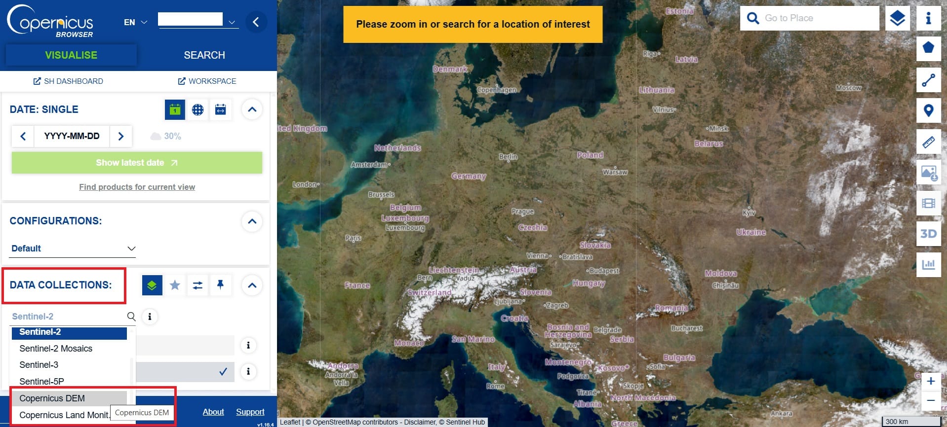
1. First, in the ‘Data Collections’ tab we select > ‘Copernicus DEM’.
2. Then we zoom-in to the area we want to download data. This time we ‘travel’ to Austria!
3. Next, on the right toolbar, we select the polygon button and we press > the rectangle button for drawing a rectangle area.

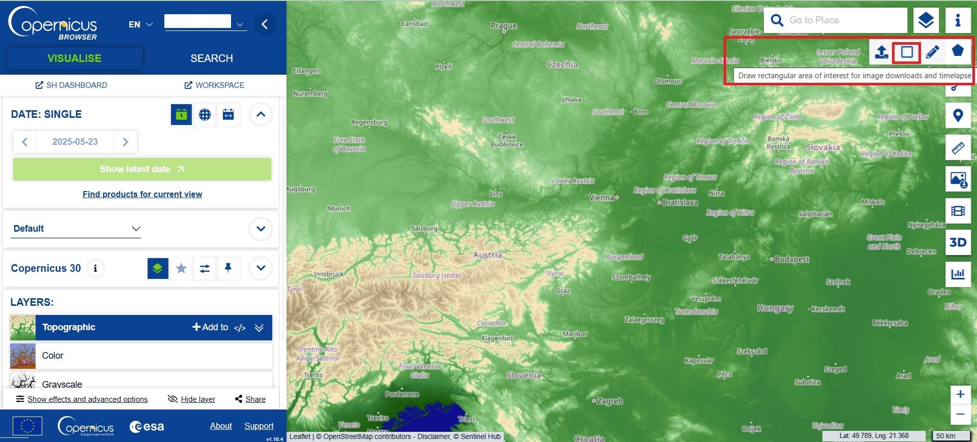
Let’s try to draw a rectangle including both mountaneous and flat areas (that’s easy in Austria)! We may draw a polygon including Vienna and the south-west part of Austria including Innsbruck, Styria, and Salzburg.

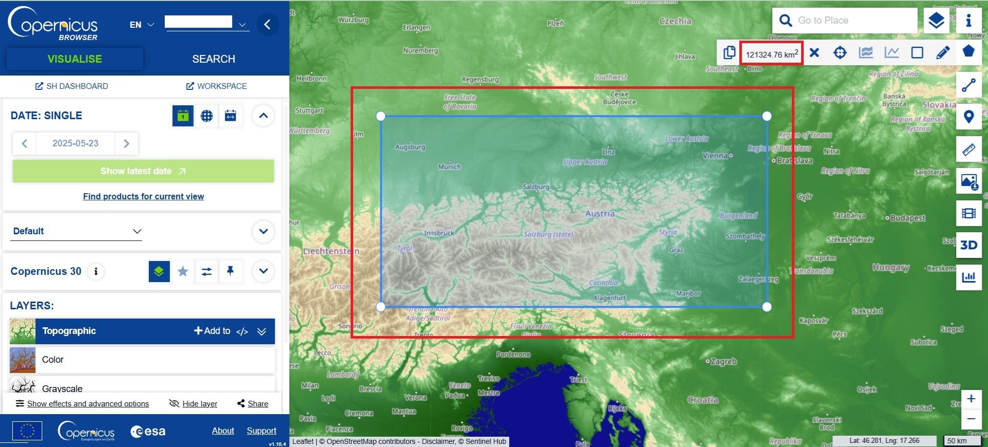
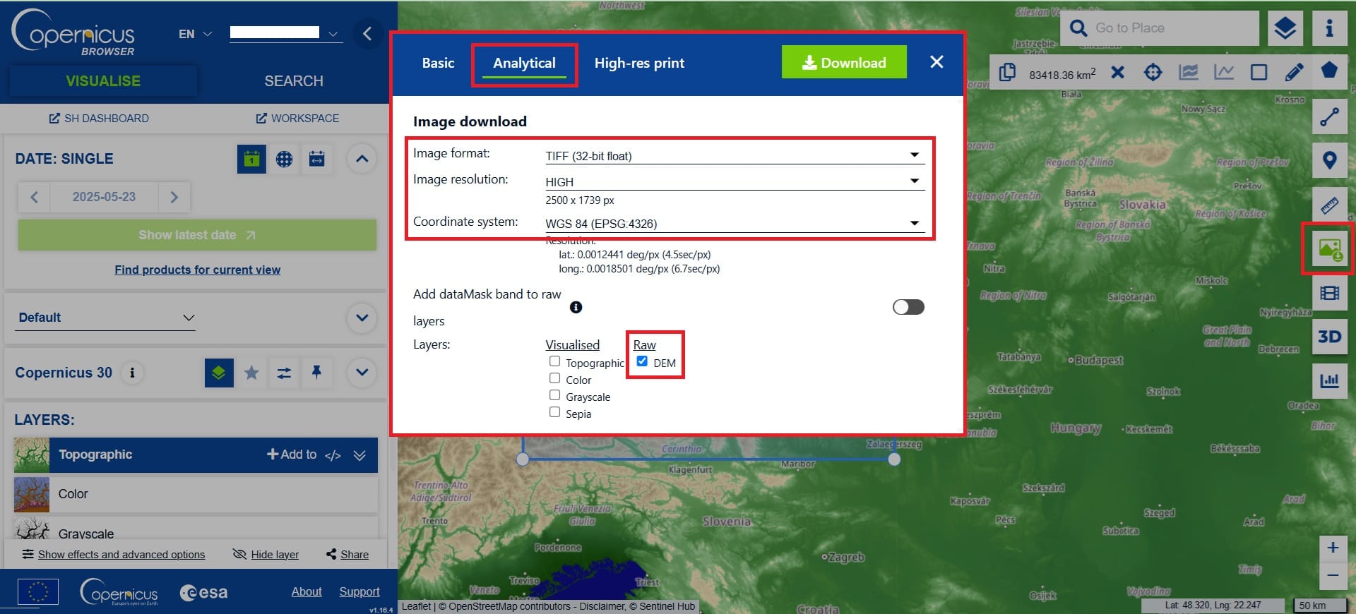
Then we select the ‘Image’ button on the right toolbar (see the image below) and a new window appears:

1. We select the ‘Analytical’ tab
2. Image format: TIFF (32-bit float since we have elevation values with decimals)
3. Image resolution: HIGH (it doesn’t matter for raw data but, if we download a .jpeg file from ‘Basic’ tab, probably we need the highest resolution possible)
4. Coordinate system: WGS 84 (EPSG 4326, what else)
5. Layers: We check the ‘Raw’ > DEM box
6. We press ‘Download’

Now you can easily guess what is the next step. Of course we open QGIS platform, we create a new project and we save it as ‘Austria’ in the ‘GIS Training’ folder. Then we copy the .tiff image we’ve downloaded to the same folder!

To load the .tiff image of Austria, we select on the main toolbar of QGIS > ‘Layer’ > ‘Add Layer’ > ‘Add Raster Layer’ and we navigate to our folder! You may also load the OSM Basemap like in the previous exercises!

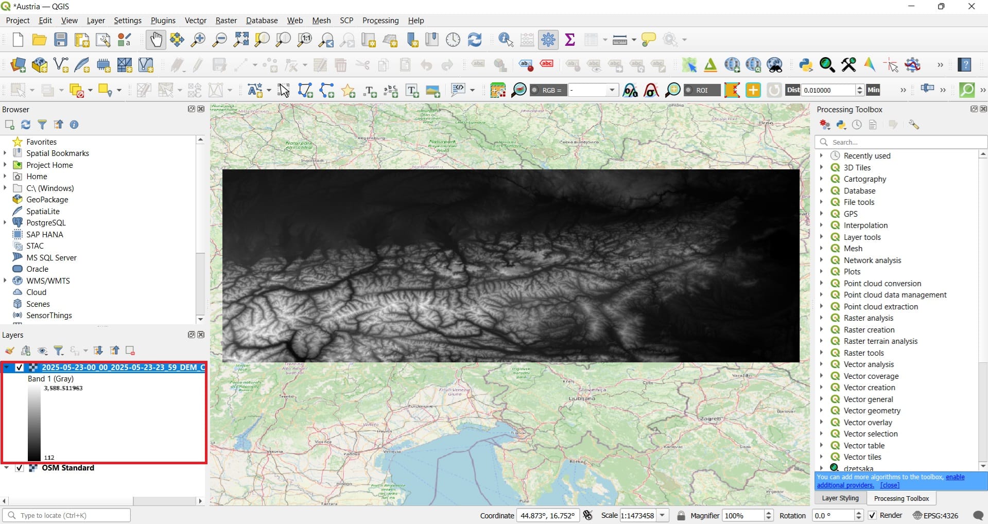
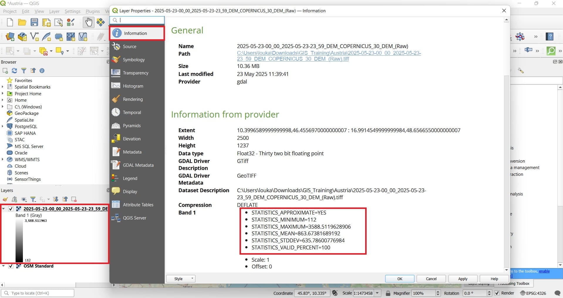
Question no.1: for you and your students: What is the minimum and the maximum elevation (in meters) of the area we’ve downloaded? Check the image above (Layers tab). As it seems, the lower-altitude areas have a minimum value of 112 meters and the high-altitude areas (the Alps) have a maximum value of 3588 meters!

Question no.2: Did we manage to download the highest altitude area in Austria? As it seems, unfortunately no since the highest altitude in Austria is Großglockner, at 3798 meters. It is located in the Hohe Tauern range, near the border between Tyrol and Carinthia. The Grossglockner is also the highest mountain in the Alps east of the Brenner Pass.

Question no.3: What is the average (mean) altitude of the area we’ve downloaded? Let’s check the raster statistics by double-clicking on our .tiff file in the ‘Layers’ tab > ‘Information’ tab! In the image below, we can see that the mean altitude value is 863 meters!

Question no.4: What is the altitude of all Austrian cities? Ok, that’s a bit more difficult but not impossible! We need some additional spatial information. All cities in Austria! How can we download all the cities? Using the SimpleMaps website (see the image below).

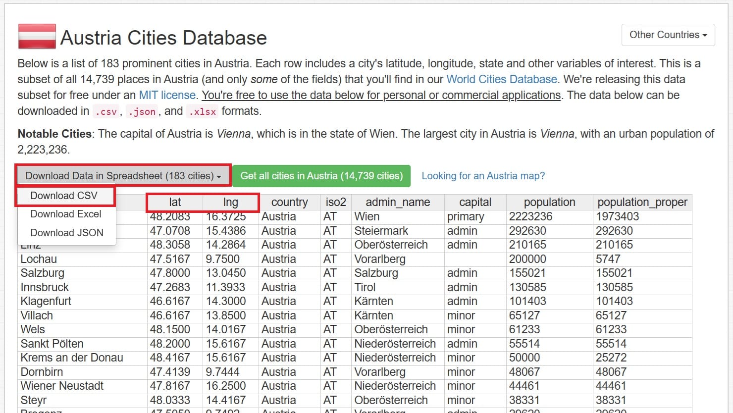
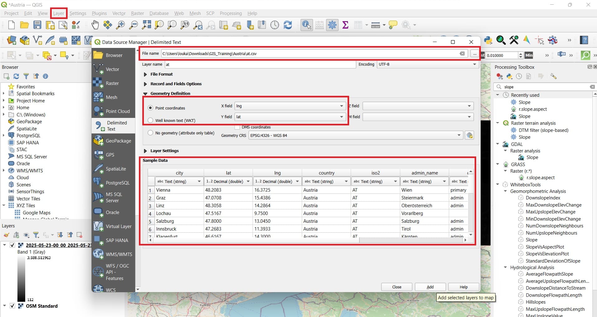
We may download all Austrian cities as a .csv delimited file (does it remind you of something?). We select ‘Download CSV’ and we copy the file to our ‘Austria’ folder. Then in QGIS we select ‘Layer’ on the main toolbar > ‘Add Layer’ > ‘Add Delimited Text Layer’.

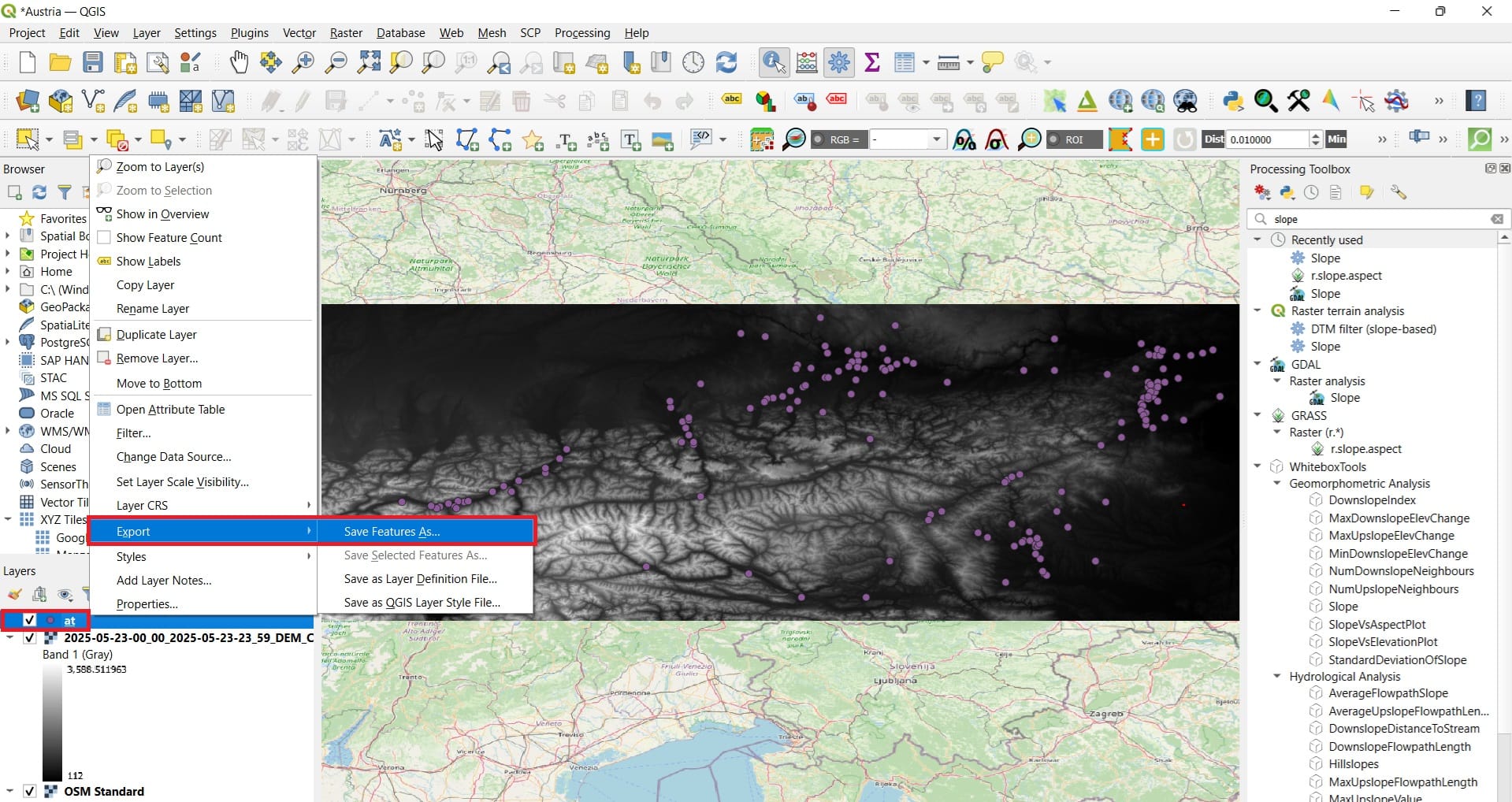
After we press ‘Add’ and we load the data, we right-click on the ‘at’ layer (Layers tab) > ‘Export’ > ‘Save Feature As’ to save it as point shapefile with the name ‘Cities_Austria’!

That was it, now we have the cities in Austria and the elevation values (DEM)! In order to find the altitude that each city is located, we need to co-locate the points we the elevation value of the pixel below each city. To do that, we will use the tool ‘Sample raster values’.

If you press on the search bar of ‘Processing Toolbox’ ‘Point sampling’, the tool will appear (see the image below).

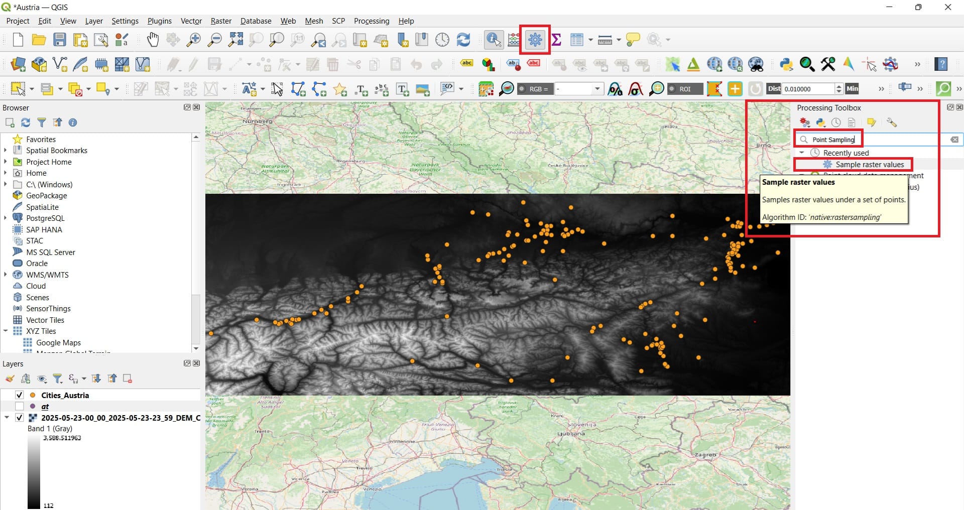
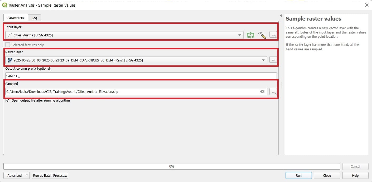
We select:

• Input layer: Cities_Austria
• Raster layer: the elevation raster (…..30_DEM_(Raw))
• We save the result as ‘Cities_Austria_Elevation’
• We press ‘Run’

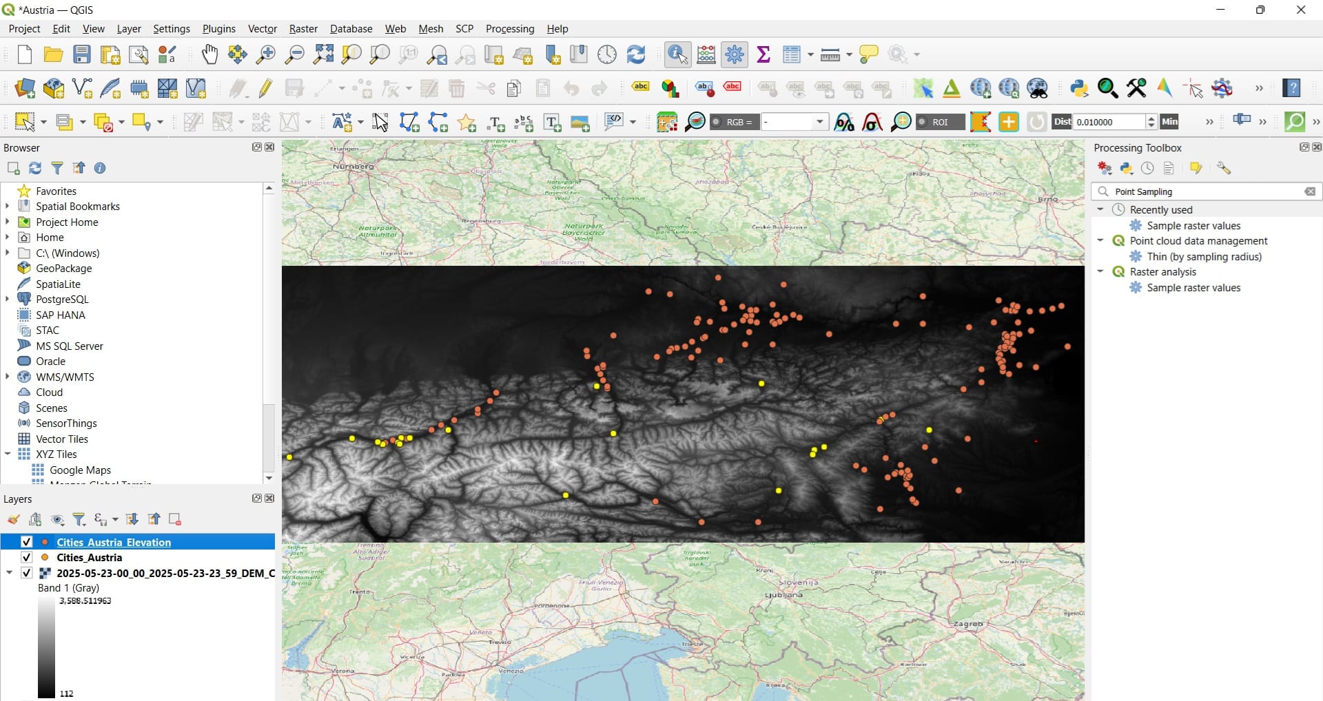
We don’t see any change on the resulting points however, if we right-click on ‘Cities_Austria_Elevation’ > ‘Open Attribute Table’, we will see that a new column has been added with the name ‘SAMPLE_1’. That’s the elevation values per city!

Thus, now we now that Vienna has an elevation of 192 meters, Graz 363 meters and Innsbruck 584 meters!

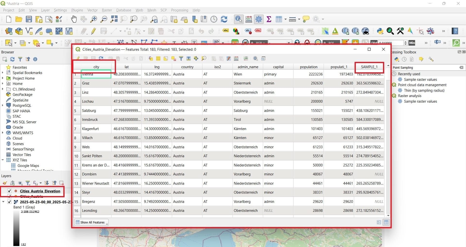
But, why some areas heve no value (NULL)? If you zoom-out, you’ll find out that the DEM raster is not covering all Austrian cities, hence, some of them fall outside the raster boundaries and there is no pixel value below to extract!

We may set some queries (questions) using the Table information. If you select ‘Select/filter features using form’ a new window will appear (see the image below)

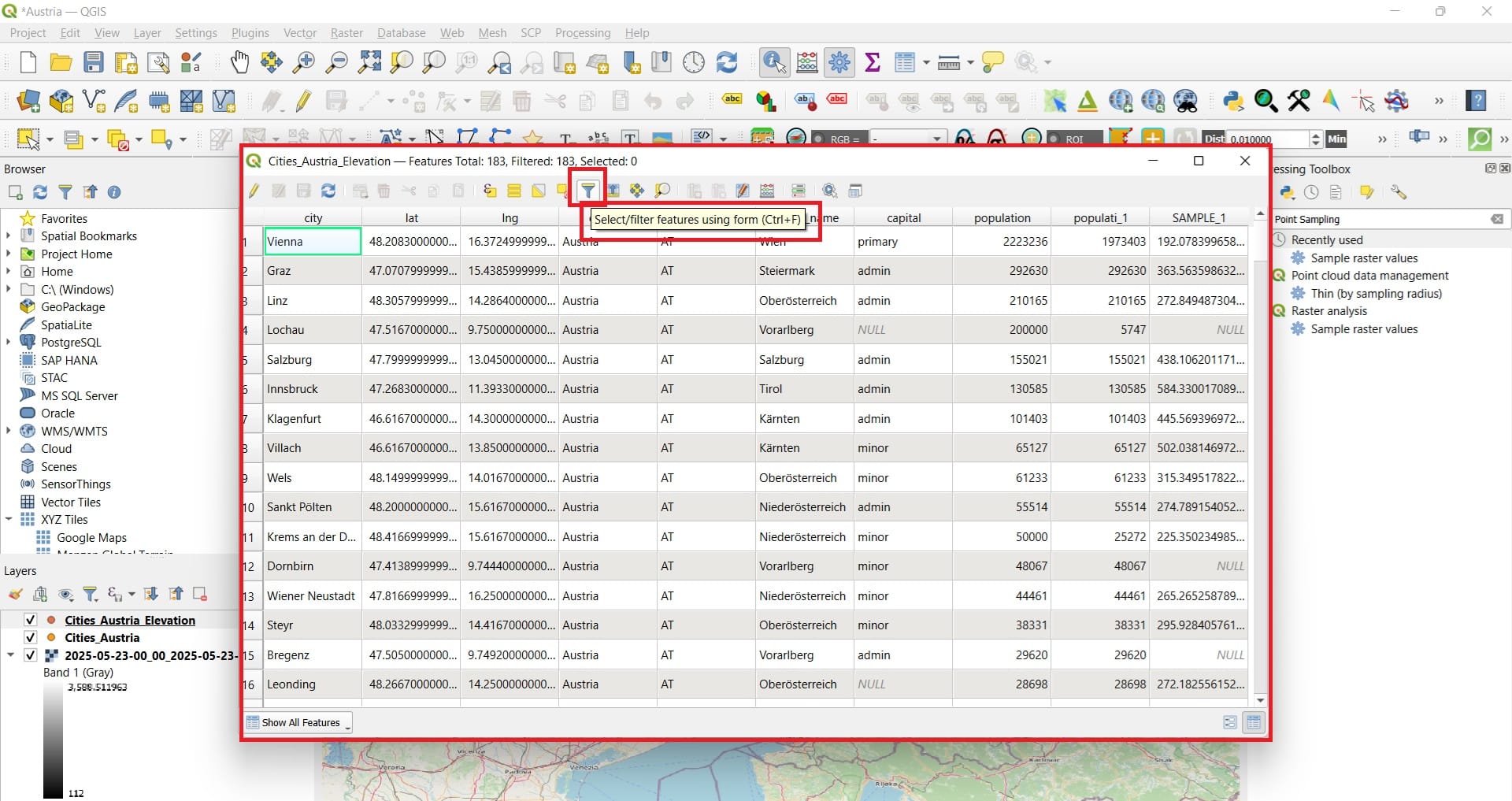
On the new window, we can ask for the cities that have a ‘SAMPLE_1’ value ‘Greater than’ 600 meters (see the image below). Then we press ‘Select Features’.

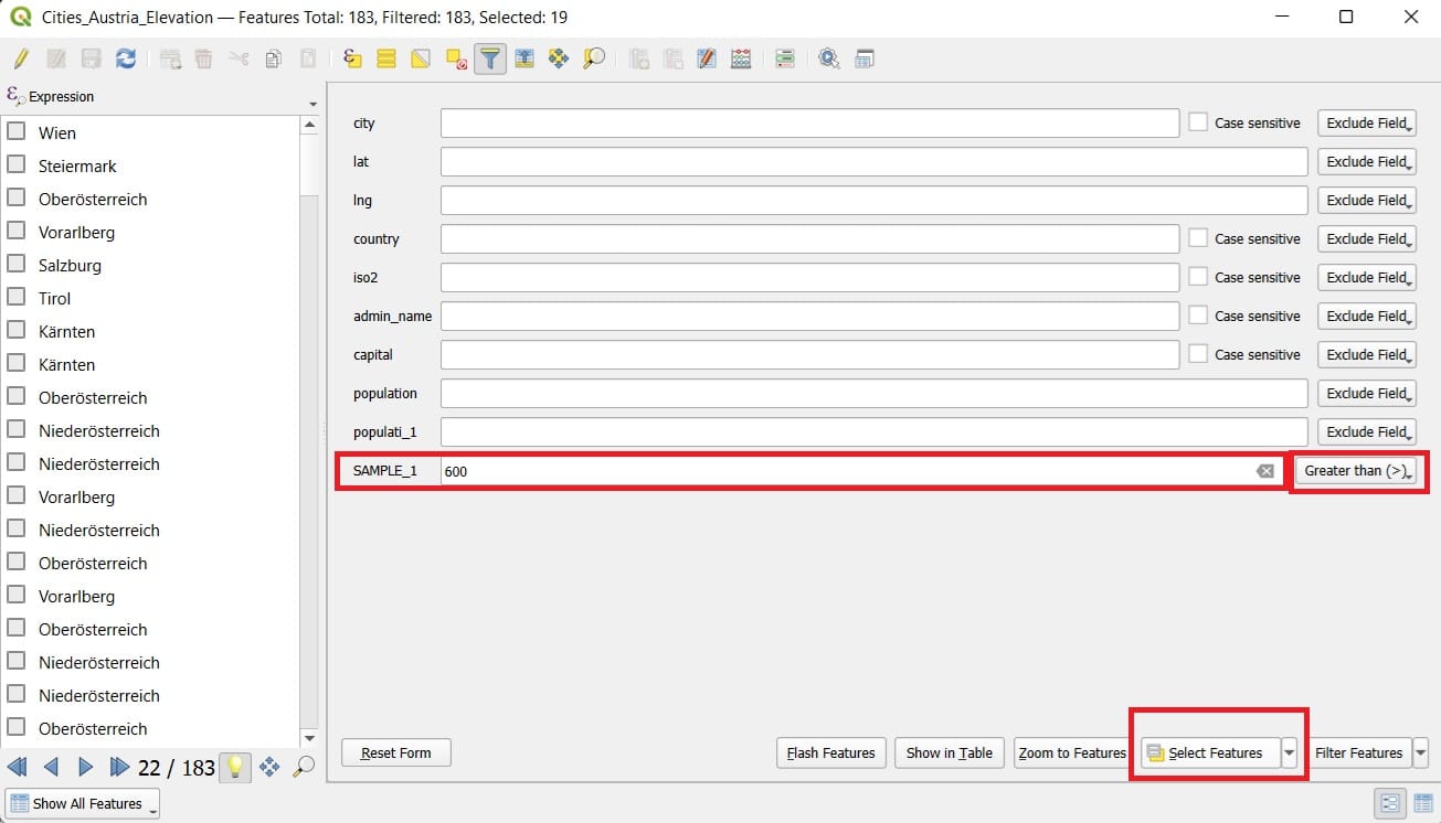
The window changes and we see the selected cities (from the left panel list with yellow if we scroll down), for example, Kpfenberg, Steienmark, Tirol etc. By pressing on each one of the cities (not the yellow box), the right panel shows us all descriptive information.

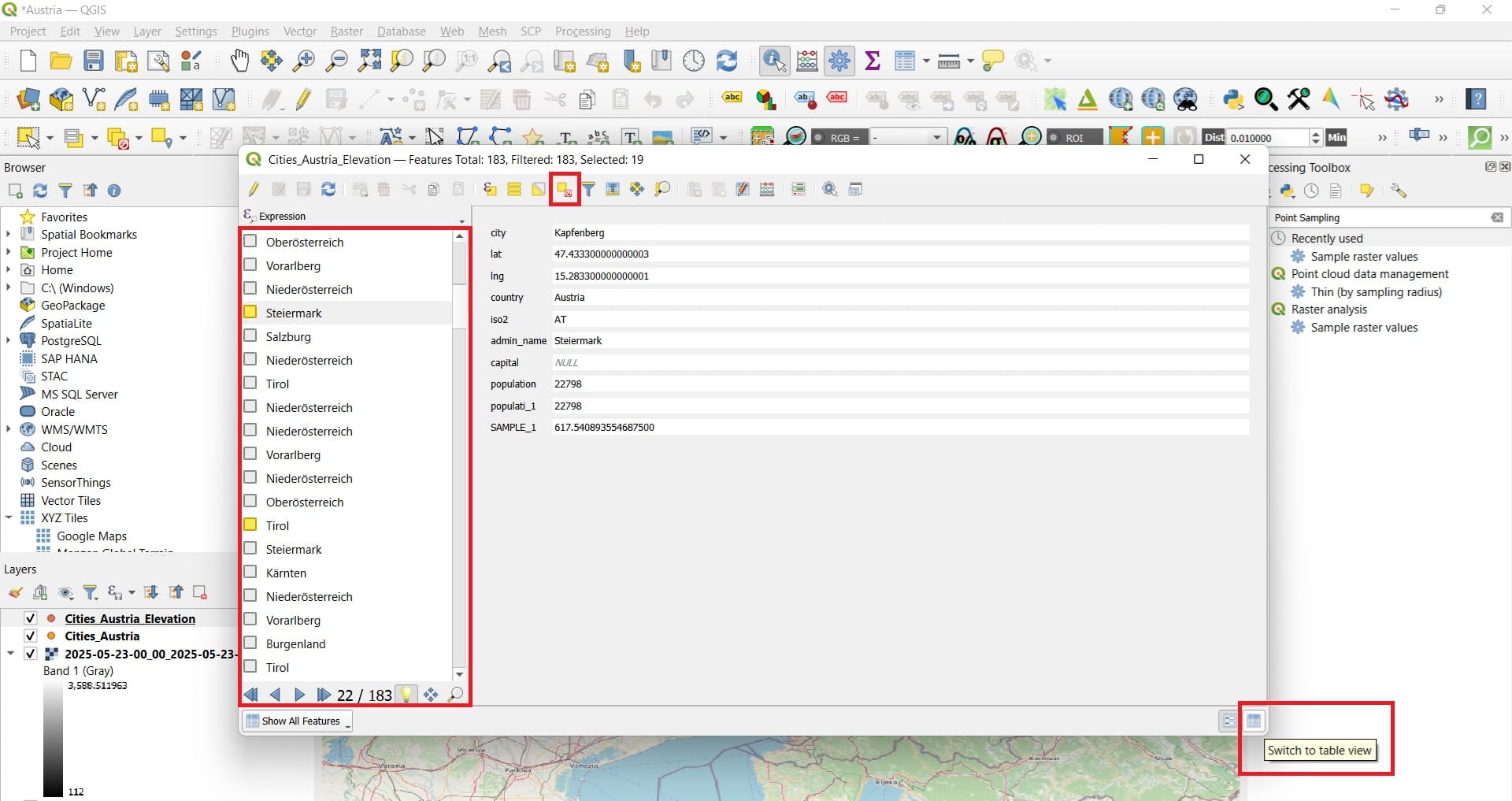
We may also see the selected cities if we minimize the ‘Attribute Table’ After we write down our results, we press the ‘Clear Selection’ button on top and then ‘Switch to Table view’ on the bottom right corner (see the image below).

Then, we may perform another query or move forward to our next question!

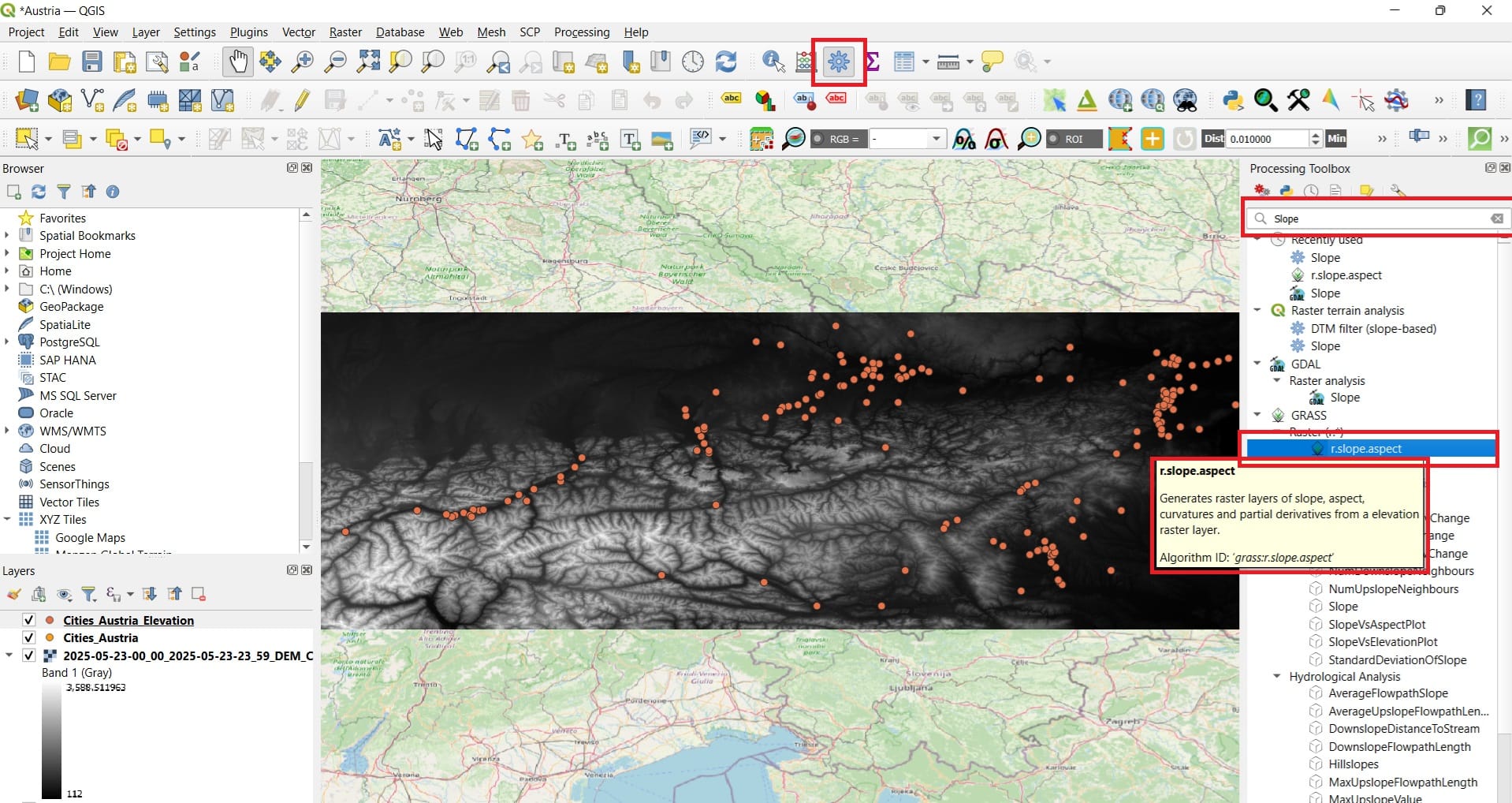
Question no.5: What is the slope and the aspect (orientation) of each city? Are they located on steep slopes, on flat areas? Do they have an orientation towards the noth or the south?

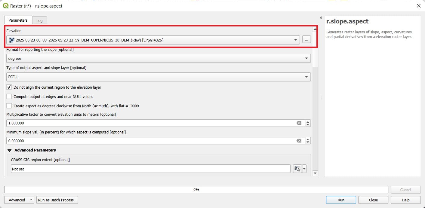
To answer these questions, we need one more tool for estimating the slopes and the aspect, based on our DEM raster file! If we search in the ‘Processing Toolbox’ toolbar for ‘Slope’, different tools will appear. The one we are going to use is the ‘r.slope.aspect’!

In the ‘r.slope.aspect’ we select:

• Elevation: the elevation raster (…..30_DEM_(Raw))
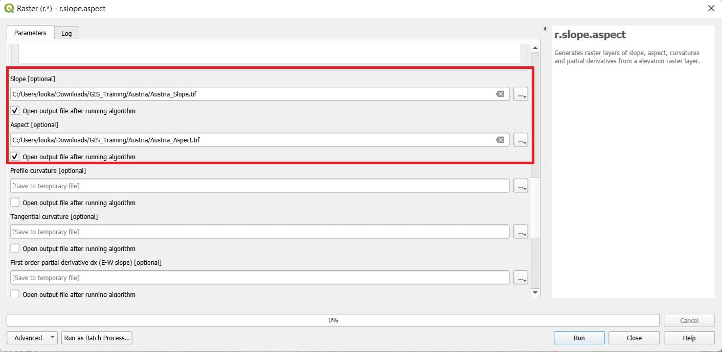
• We scroll down and we uncheck all boxes except for ‘Slope’ and ‘Aspect’ where we save them as ‘Austria_Slope’ and ‘Austria_Aspect’ (see the images below)
• We press ‘Run’

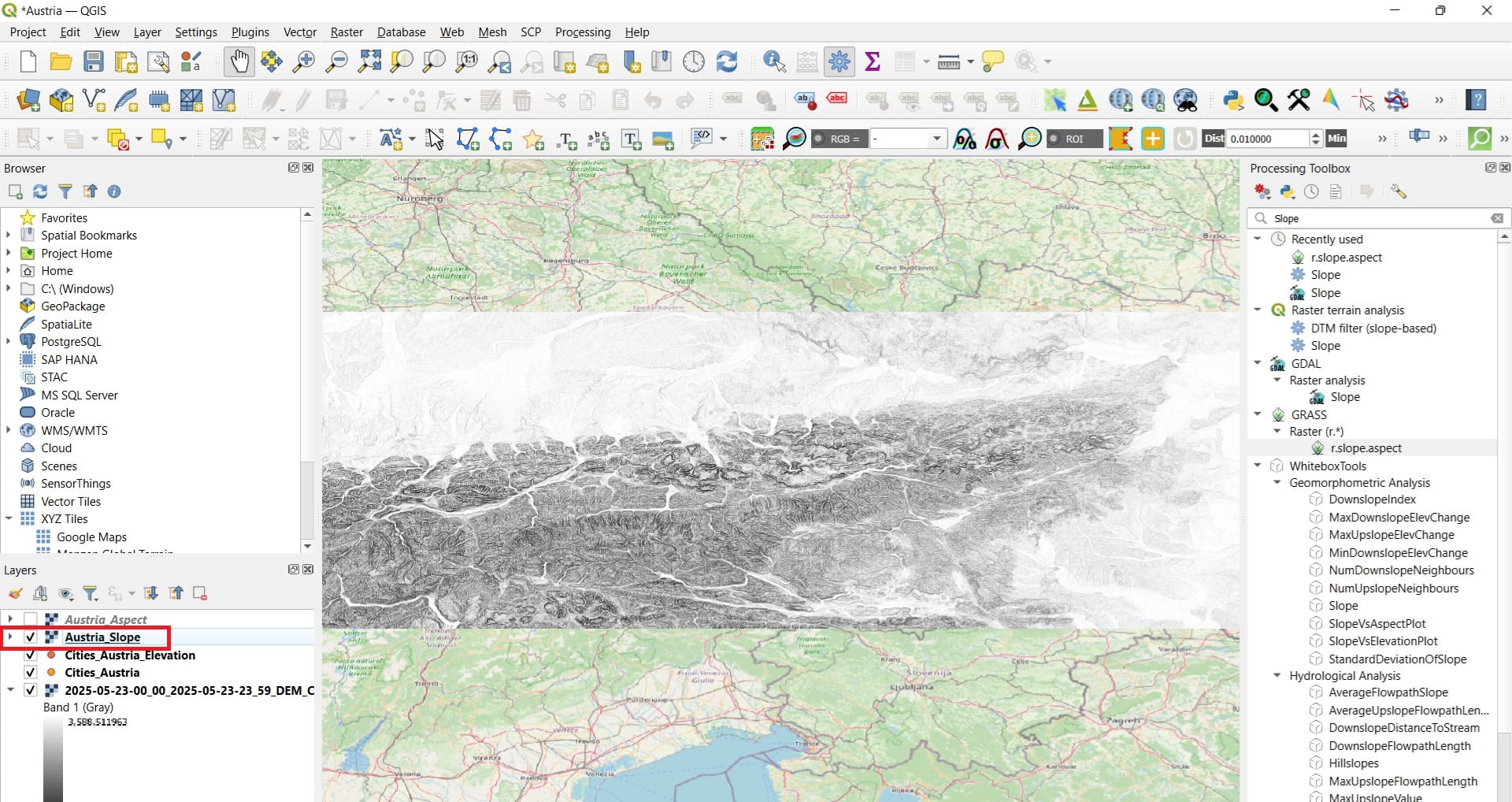
The resulted rasters will look like this…

Aspect

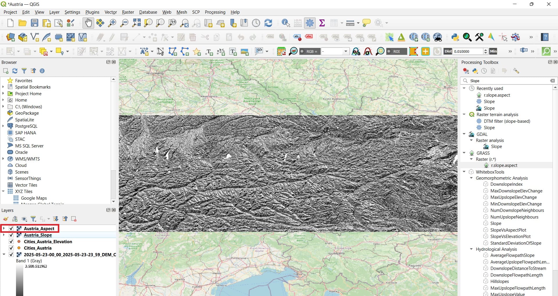
Slope

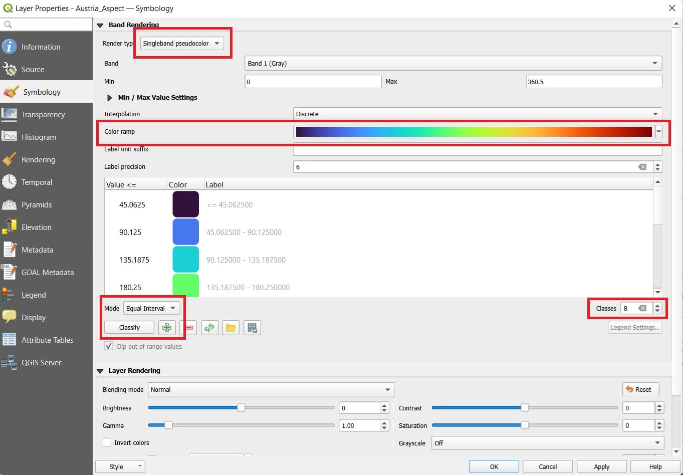
Let’s make the images more impressive by changing the colors via the ‘Symbology’ > ‘Singleband Pseudocolors’ > We select the ‘Turbo’ color ramp! Also, we set:

• Mode: Equal interval (on the left below the window)
• Classes: 8 on the right below the window
• We press ‘Classify’ and OK
• We repeat the same process for the ‘Austria_Slopes’ file

The new colors and the classes we’ve created will look like this:

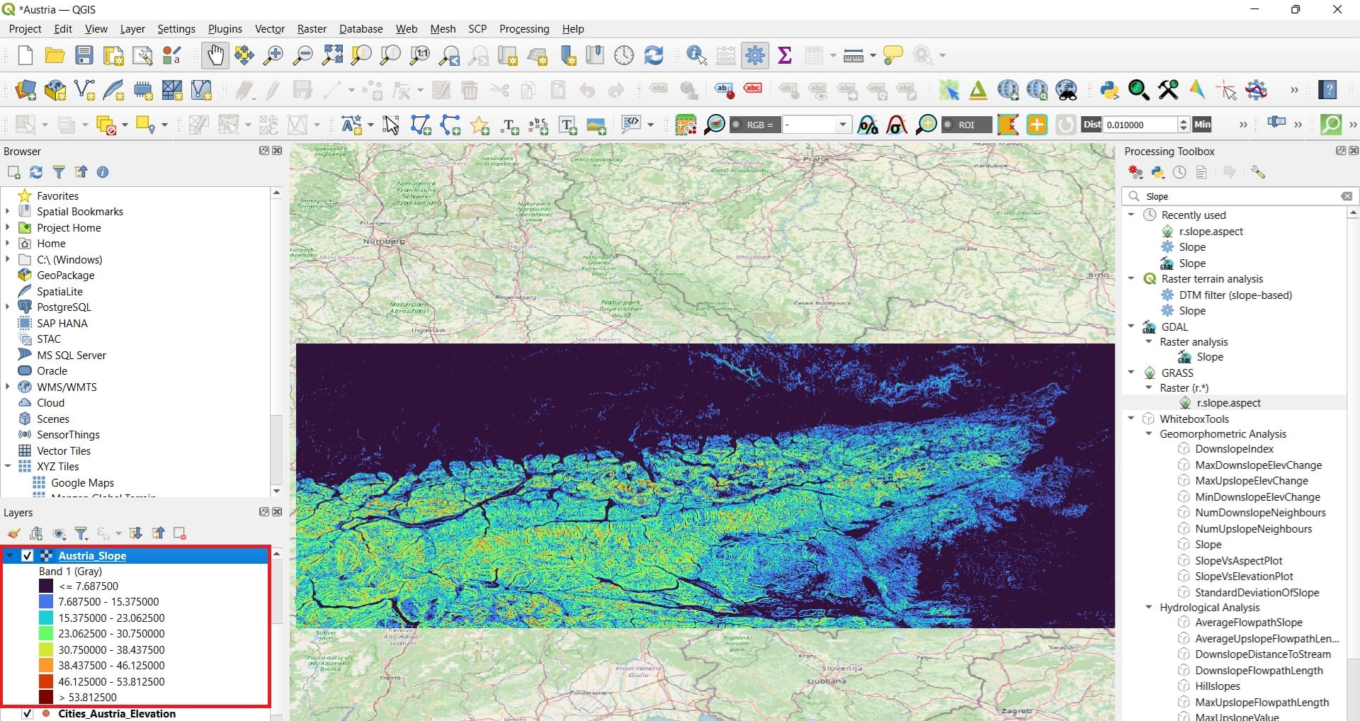
Slopes

This map visualizes the steepness of the terrain, calculated in degrees, using the DEM. Slope values show how inclined the land is at any given location. The Color Gradient indicates:

• Dark Blue to Light Green (< 7° and 7° – 23°): These areas represent flatter terrain—valleys, plains, or gently sloping hills.
• Yellow to Orange (23° – 46°): These are moderate slopes, likely representing rolling hills or the lower slopes of mountain ranges.
• Red to Dark Brown (46° – 53° and >53.81°): These areas represent very steep terrain, such as mountain ridges, cliffs, or escarpments—common in the Austrian Alps.

This slope analysis is useful for applications such as construction planning, soil erosion risk, and route planning in mountainous areas.

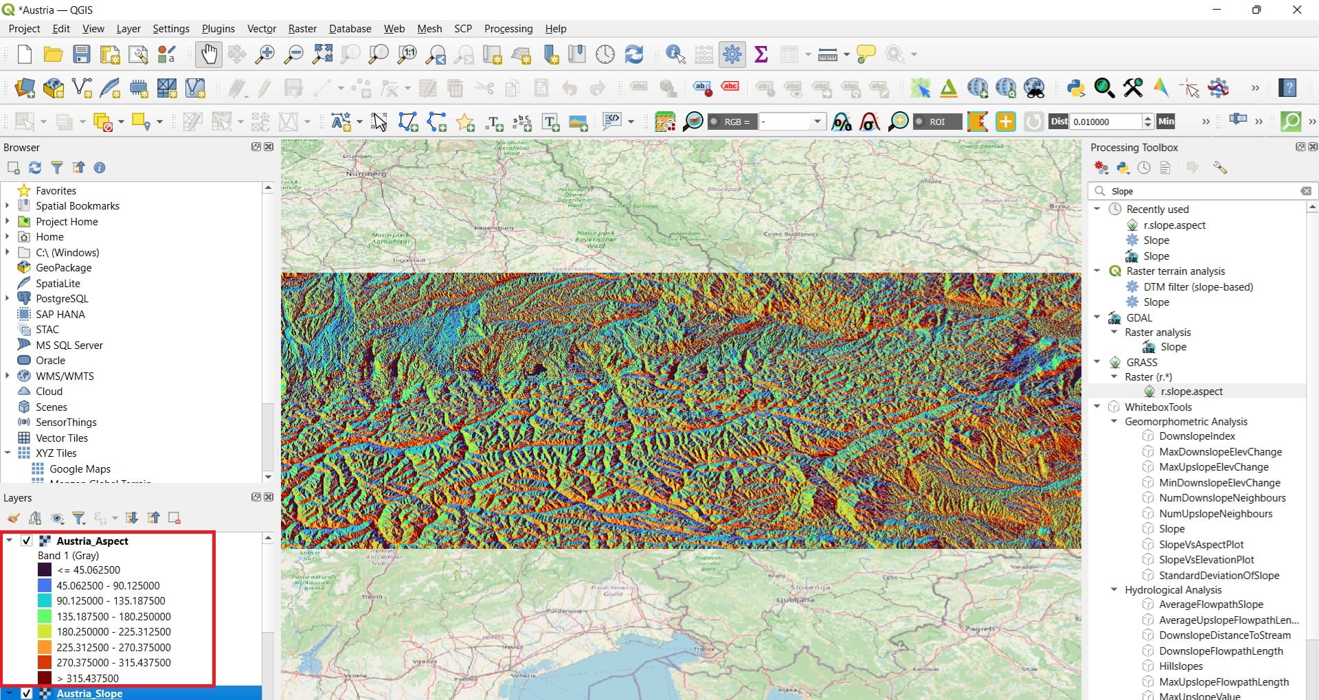
Aspect

This map represents the orientation or direction that each slope faces—also known as the “aspect” of the terrain. The Color Coding indicates:

• Blues and Purples (<90°): Represent slopes facing north to east.
• Greens to Yellows (90° – 180°): Represent east- to south-facing slopes.
• Oranges to Reds (180° – 315°): Represent south to northwest-facing slopes.
• Dark Red to Brown (>315°): Represent slopes facing back toward the north.
• Dark Purple or Black: Indicates mainly flat areas with no slope or undefined aspect.

Aspect is crucial in fields such as agriculture (sun exposure), ecology (vegetation patterns), solar panel siting, and microclimate studies.

Similarly to the elevation extraction for the Austrian cities, we  may find the slope and the aspect that each city is located. We simply need to co-locate the points we the slope and aspect values of the pixels below each city. To do that, we will use again the tool ‘Sample raster values’.

You may also take a look on the following video, explaining how to use the QGIS surface analysis tools!

✅ Wrapping Up: Raster Processing – Surface Analysis

You’ve now completed the “Raster Processing – Surface Analysis” course, where we explored how to use QGIS to extract valuable information from elevation data. This lesson marked a major step in understanding how raster datasets—particularly Digital Elevation Models (DEMs)—can help us better analyze the landscape around us. Throughout the course, we:

✅ Worked with the Digital Elevation Model (DEM) of Austria, learning how elevation data is structured and how it provides the foundation for topographic analysis.
✅ Calculated slope values to measure how steep the terrain is in different regions. We learned how steep slopes might impact land use, erosion, construction, or natural hazard risk.
✅ Generated aspect layers to determine the orientation of slopes (i.e., which direction each slope faces). This helped us understand sunlight exposure, climate variation, and landscape patterns.
✅ Visualized the results with color-coded maps, using legends to interpret terrain variation—from gentle valleys to steep alpine ridges.
✅ Zoomed in on specific cities in Austria to observe how the local terrain (slope and aspect) might affect urban planning, transport infrastructure, or environmental conditions.

These techniques are essential for a wide range of real-world applications, such as:

• Land suitability analysis
• Disaster risk management
• Infrastructure development
• Renewable energy siting
• Environmental education and fieldwork preparation

By mastering slope, aspect, and DEM-based analysis, you now have the tools to extract meaningful terrain data and use it for informed spatial decisions.

In the next course, we’ll take this further by applying what you’ve learned to perform more advanced analyses, including least-cost path modeling, multi-criteria site selection, and 3D terrain visualization.

Well done—and keep exploring the power of spatial data! 🌍🗺️📈

Useful links

1. USGS: What is a digital elevation model (DEM)?
2. Eurostat: Digital Elevation Model (DEM)
3. NASA: Digital Elevation/Terrain Model (DEM)
4. QGIS: Lesson: Terrain Analysis
5. Kings College London: Aspect-Slope analysis in QGIS