Multi-criteria problem-solving

🧭 Introduction to Multi-Criteria Problem-Solving in QGIS

In the previous lesson, we explored fundamental raster processing techniques—clipping rasters, filling NoData values, and converting vector data to raster format. These steps have equipped us with the essential tools to delve into more complex spatial analyses.

Now, we’re ready to apply these skills to perform a Multi-Criteria Overlay Analysis (MCDA). This method allows us to evaluate multiple spatial criteria simultaneously to identify optimal locations for specific objectives. For instance, in the context of planning an Offshore Wind Energy project, we’ll assess various factors such as wind speed, proximity to infrastructure, and environmental constraints to determine the most suitable sites.

By the end of this lesson, you will:

✅ Understand the principles of Multi-Criteria Overlay Analysis in a GIS context
✅ Combine multiple raster layers representing different criteria into a single suitability map
✅ Apply weighting schemes to reflect the relative importance of each criterion
✅ Utilize QGIS tools to perform raster calculations and generate composite analyses

This lesson will demonstrate how the raster processing techniques you’ve learned can be integrated into a comprehensive analysis framework, enabling you to tackle real-world spatial decision-making challenges effectively.

Let’s dive into this journey to transform processed data into actionable insights! 🌍📊🗺️

🌍 Before we start, let’s explain what Multi-Criteria Analysis is!

Multi-Criteria Analysis (MCA) within a Geographic Information System (GIS) is a technique that helps decision-makers evaluate and compare different spatial alternatives based on multiple, often conflicting, criteria. It combines spatial data with structured decision-making methods to find the best solution for a given problem, such as land suitability, risk assessments or site selection for renewable energy source like wind or solar farms [1,2].

Let’s see a few exemplary cases:

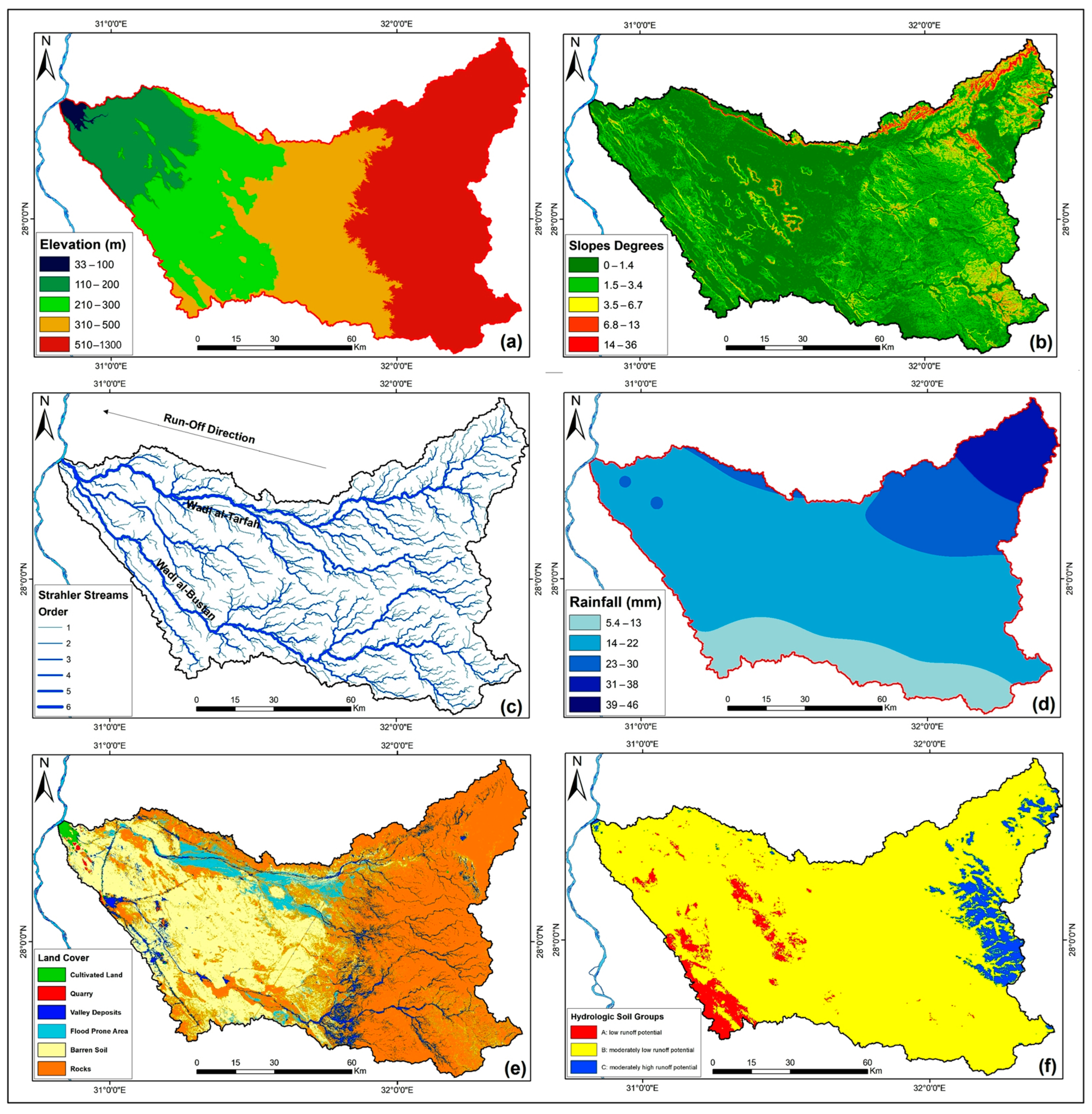
GIS-Based Multi-Criteria Decision Analysis for Flash Flood Hazard and Risk Assessment in Egypt [3]. Multi-criteria applied in this study includes different criteria for estimating Flood Hazard consisting of (see the image below): (a) Elevation (m) data; (b) Slopes (Degrees) data; (c) Streams (Rivers); (d) Rainfall data from 2010 to 2020 in mm; (e) Land use/Land cover in 2020 data; and (f) Hydrological Soil Group

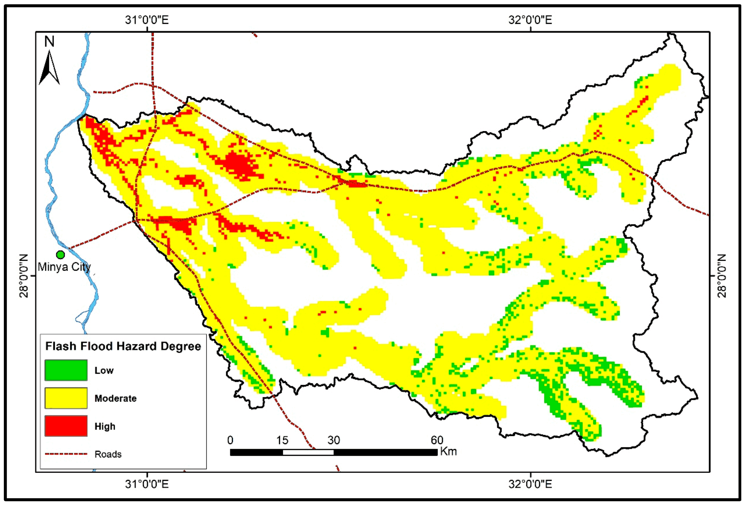
And the resulting Flood Hazard map…

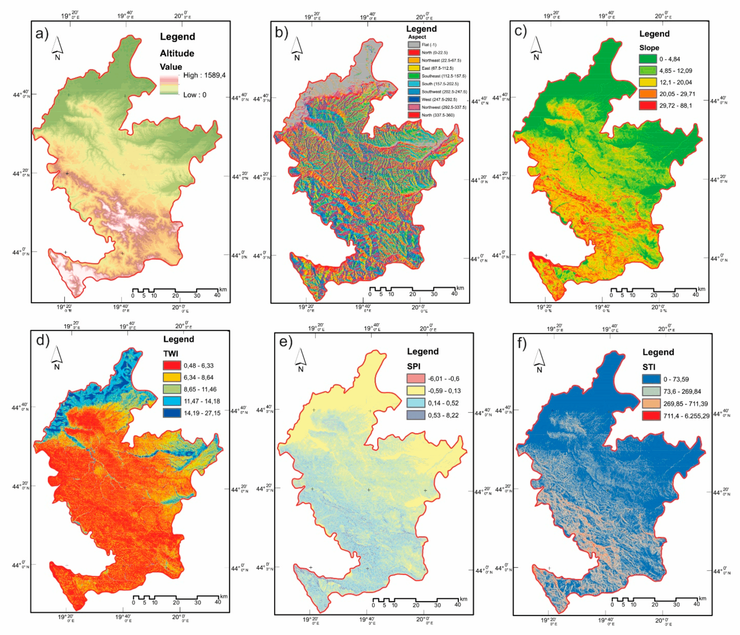
The application of a GIS Spatial Multi-Criteria Decision Analysis for Landslide Susceptibility Mapping in Serbia [4]. The topographical factors related to landslides include: (a) the elevation; (b) the aspect; (c) the slope; (d) the topographic wetness index; (e) the stream power index; (f) the sediment transport index.

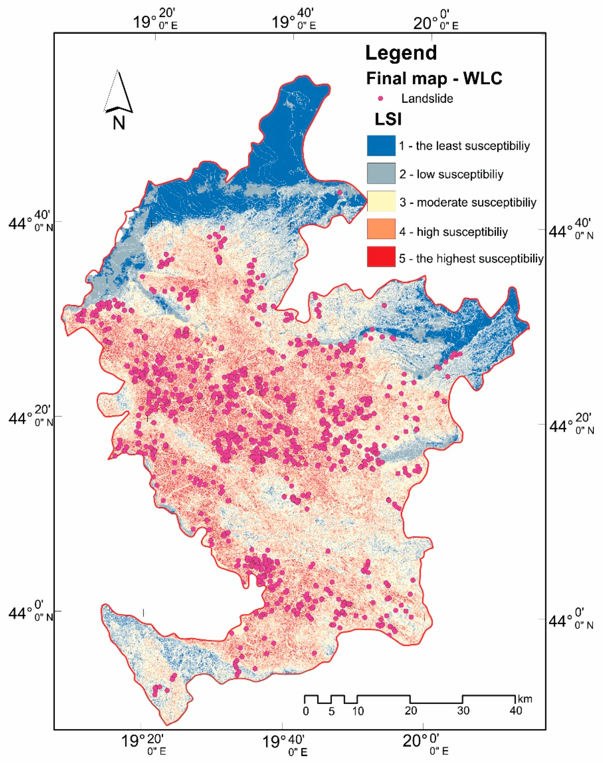
And the resulting Landslide susceptibility map looks like this…

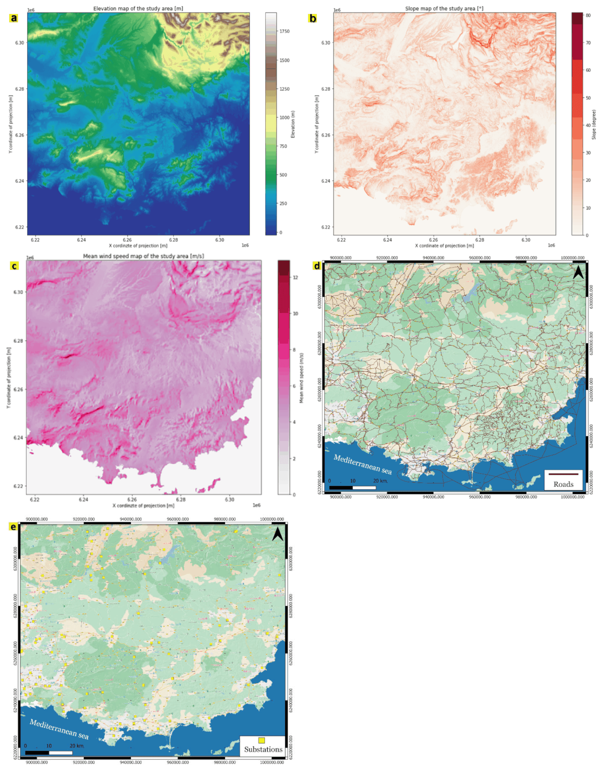
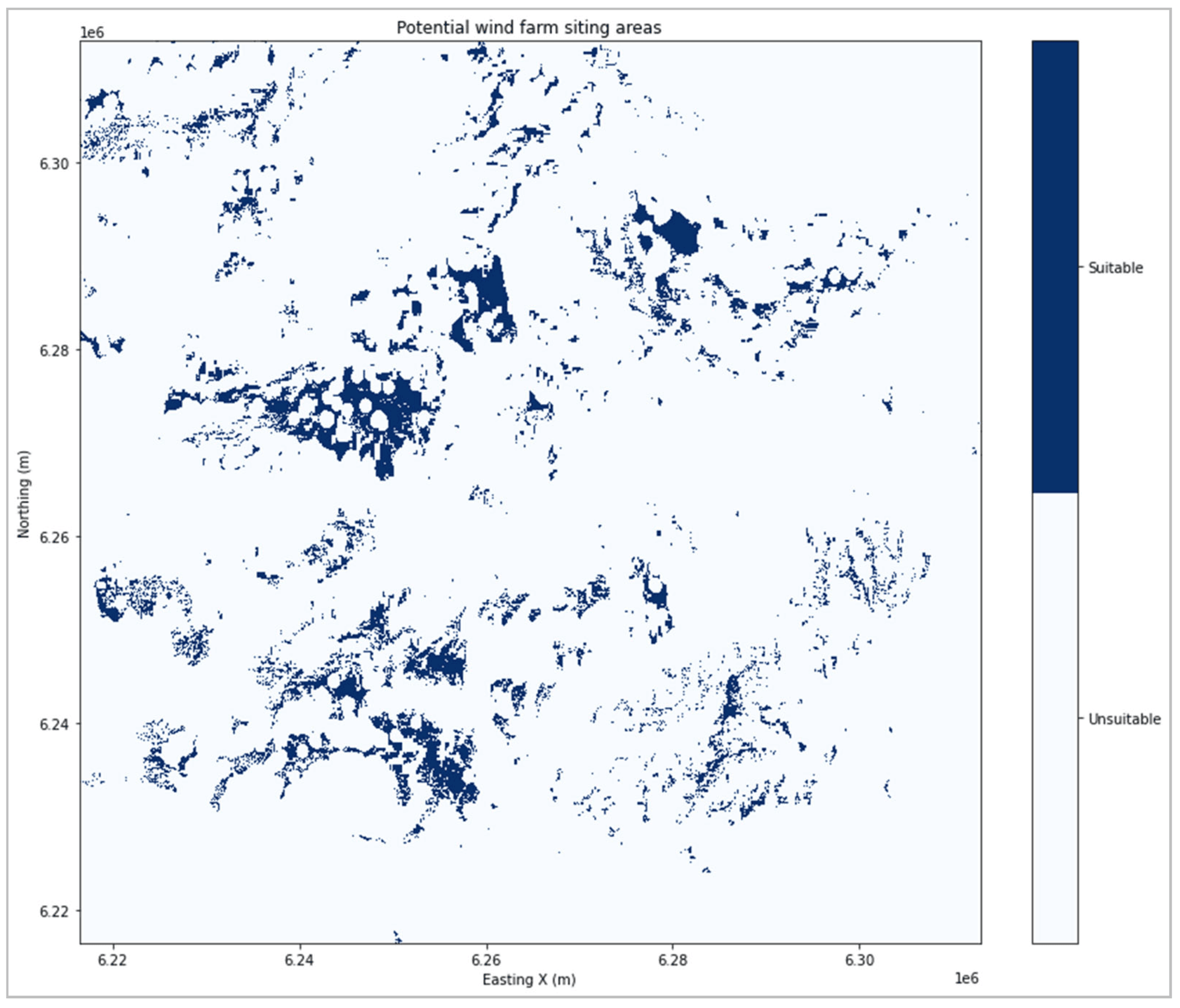
Or the Multi-Criteria GIS-Based Analysis for Mapping Suitable Sites for Onshore Wind Farms in Southeast France [5]. The criteria include the: (a) Elevation map (m); (b) average wind speed map (m/s); (c) slope map (degrees); (d) road network; (e) locations of power plants and substations in the study area.

And the resulting suitability map looks like this…

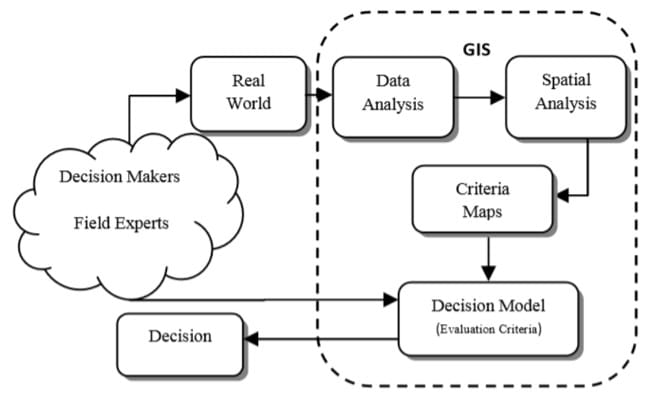
In order to solve theabove-mentioned problems, whether it’s for a hazard or a site-suitability analysis we must follow some concrete steps and a specific scientific approach! The key steps when performing a GIS-MCA incorporate (see the figure below) [1]:

1. Define your problem, goal or objective.
2. Determine the criteria and the constraints. Using a combination of experts’ opinions and information from various sources (experts of relevant fields, surveying of literature and analysis of historical data).
3. Transform the values onto a relative scale. This allows for comparison between each of the criteria, and for us to represent the judgments and expert knowledge with meaningful numbers.
4. Weight the importance of each criterion in regards to the objective, and in respect to each other.
5. Combine, synthesise and aggregate the layers/criteria together.
6. Analyse and then validate your results – Sensitivity Analysis

Which of the above-mentioned steps did we cover in our previous lesson? Only Step 3 where we transformed our vector and raster data to a common format (i.e. raster) and scale from 1-10! Let’s unfold what we were actually preparing by downloading data related to wind, sea depth and the Natura areas!

1. Step 1: Define your problem, goal or objective. Let’s find the best offshore areas for placing wind turbines (Offshore Wind Farms).
2. Step 2: Determine the criteria and the constraints. Ok, Offshore Wind Farms in the sea, hmmm. Maybe we need data related to wind and depths. Any other criteria? Ok, since renewable energy sources are environment-frindly, we may use an environmental criterion like the Natura areas.
3. Transform the values onto a relative scale. Ok, we did that already! We transformed the Natura, wind and depth data to a common scale of 1-10 so that we know for each criterio whic are the best and the worst areas!
4. Weight the importance of each criterion. We didn’t do that! Let’s try it!

These weights reflect the relative importance of each factor in achieving the overall objective. While advanced methods like the Analytic Hierarchy Process (AHP, [6]) involve detailed pairwise comparisons to derive these weights, for educational purposes, a simplified approach can be more effective and engaging. In our exercise, you and your students will determine the importance of each criterion based on informed discussions and collaborative decision-making.

Example Scenario: Offshore Wind Energy Projects in France based on wind speed, bathymetry and the Natura areas data

Let’s consider those criteria and explain why they are important for Offshore Wind turbines site-prospecting:

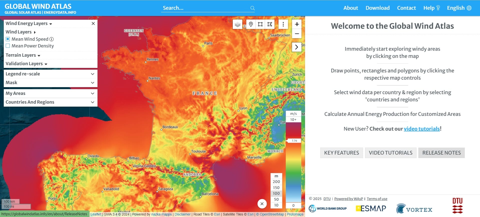
1. Wind Speed – Crucial for energy generation efficiency. Also, bigger wind turbines might be placed in windier areas and smaller wind turbines to less windy areas.
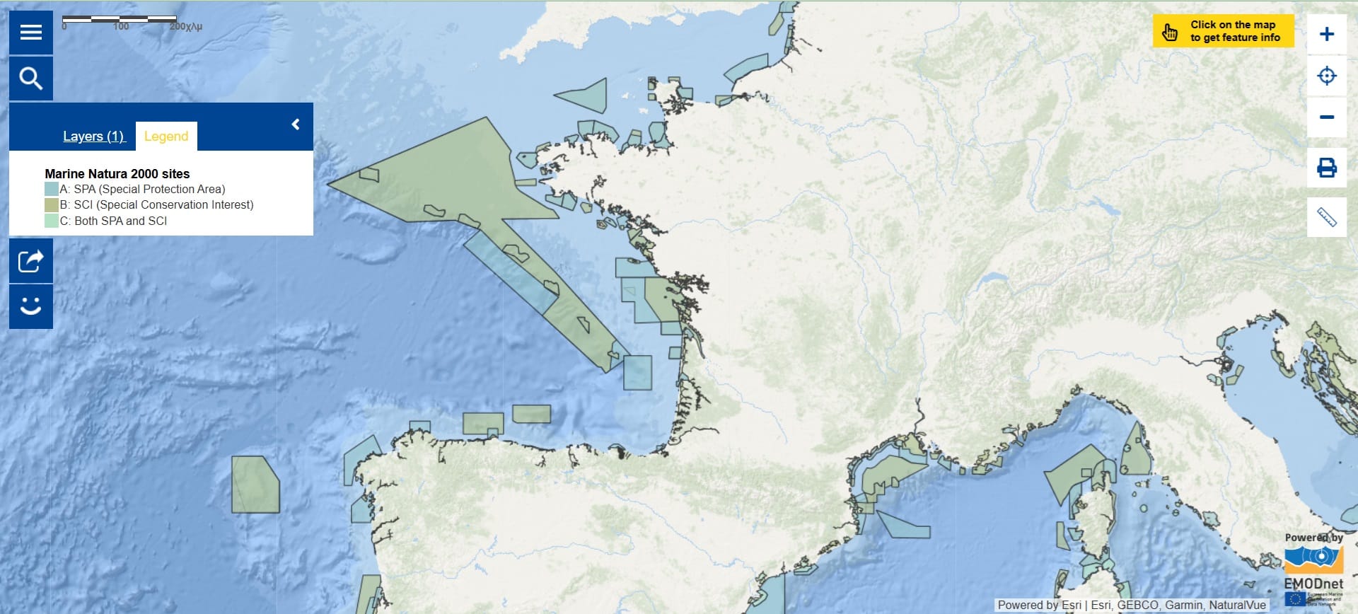
2. Natura 2000 Protected Areas – Important for environmental conservation.
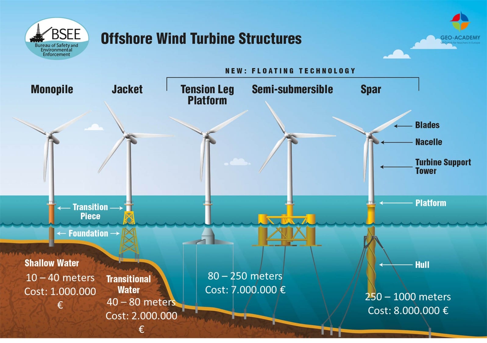
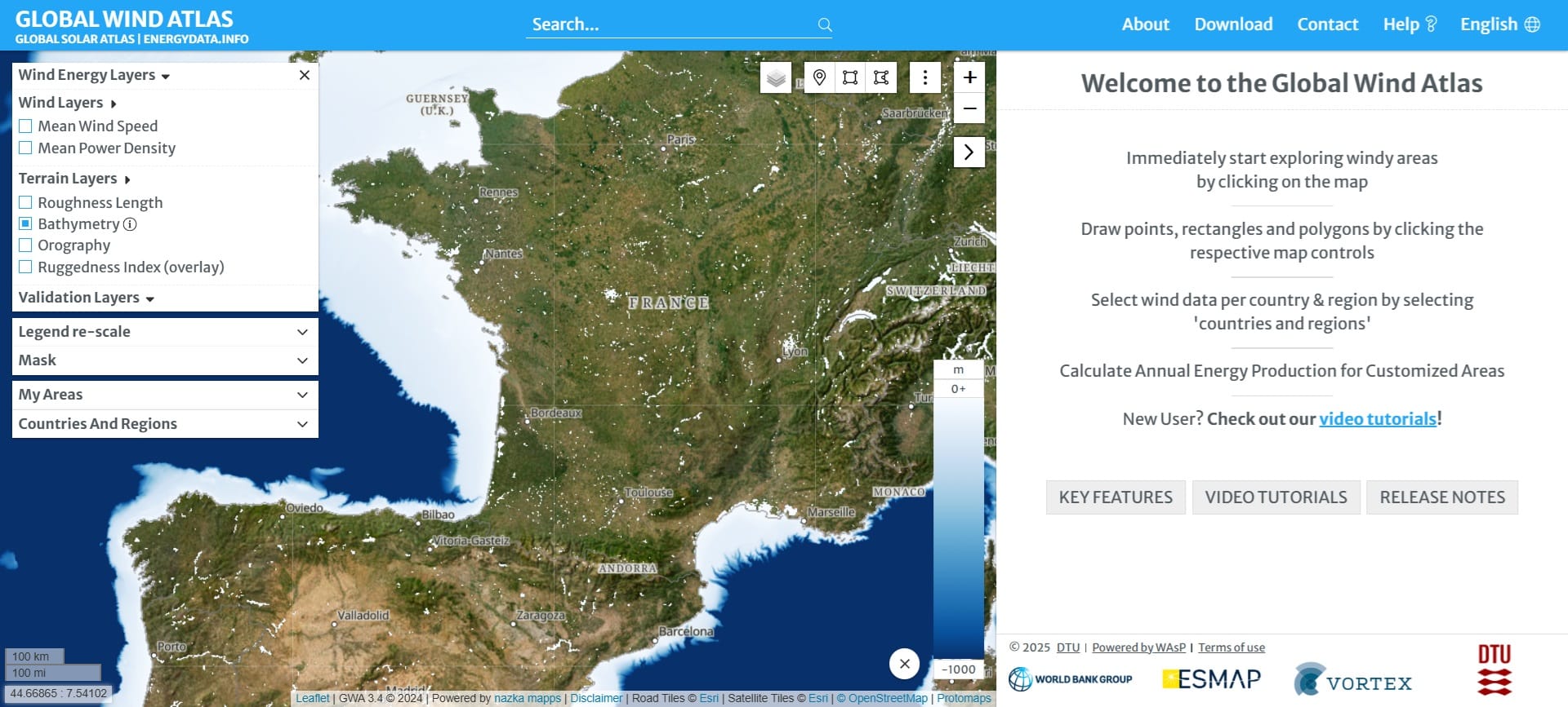
3. Bathymetry (Sea Depth) – Relevant for construction feasibility (up to 80 meters depth it’s cheaper and we use fixed foundations otherwise, beyond 80 meters we should use floating structures which is more expensive).

You may show to your students the following images to explain the above-metnioned differentiations! Also, take a look on the support material attached in this lesson.

Offshore wind turbines foundation types [7]

Offshore wind turbines size and cost evolution [7]

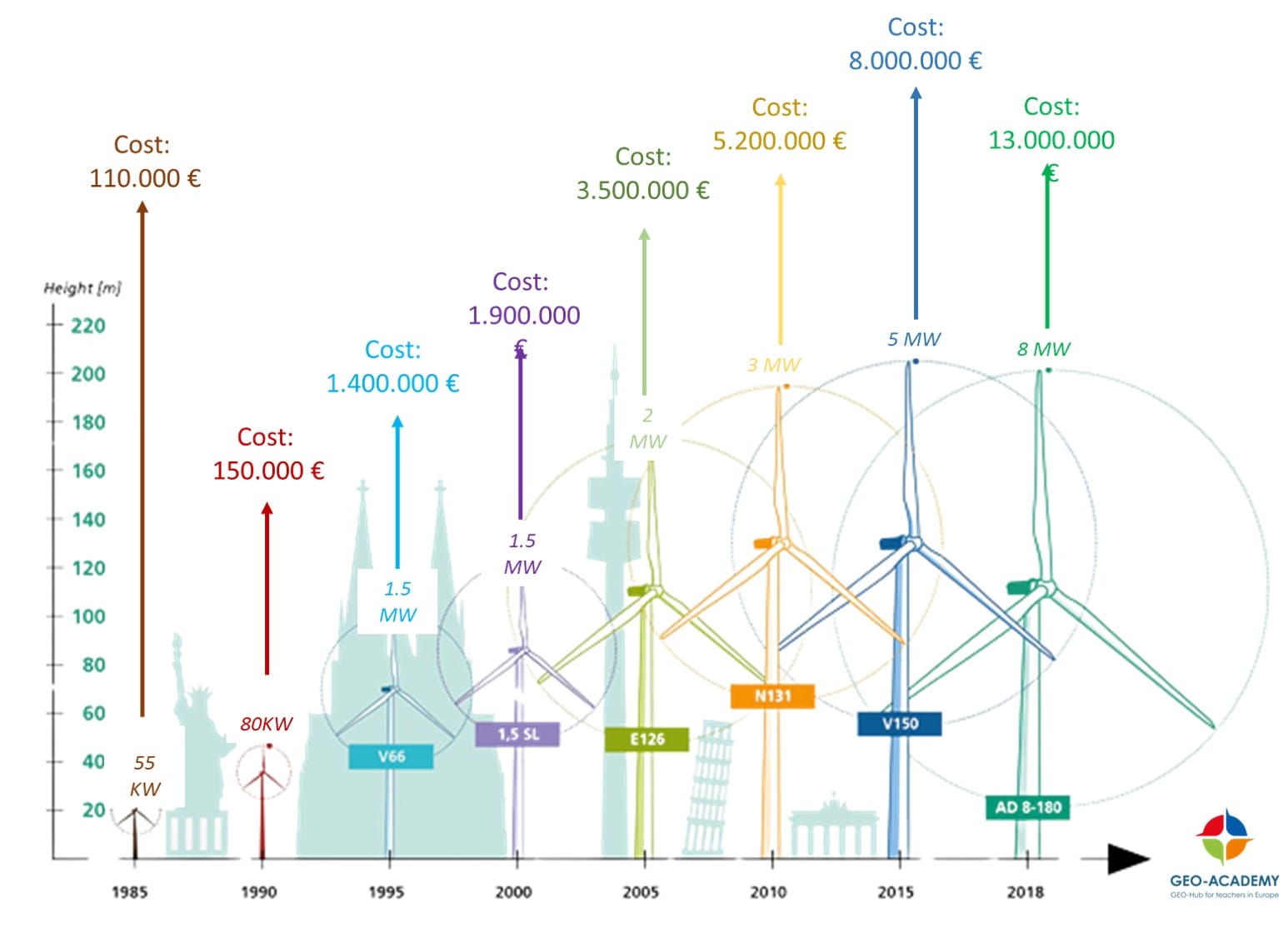
Ok, now we have all information we need! Let’s decide which criteria are the most important! Students might decide on the following weights:

• Wind Speed: 0.45
• Natura Areas: 0.35
• Bathymetry: 0.20

These weights are expressed on a scale from 0 to 1 and should sum up to 1. This ensures that each criterion’s influence is proportionally represented in the analysis. Keep in mind that by involving students in this weighting process, they gain a deeper understanding of how different factors impact decision-making in spatial analyses. This hands-on approach fosters critical thinking and allows students to appreciate the complexities involved in real-world planning scenarios.

In the next step, we’ll apply these weights using QGIS to perform a weighted overlay, combining our criteria into a comprehensive suitability map. This map will visually represent the optimal locations for offshore wind energy development based on the assigned priorities. Let’s open QGIS again and our ‘France’ project!

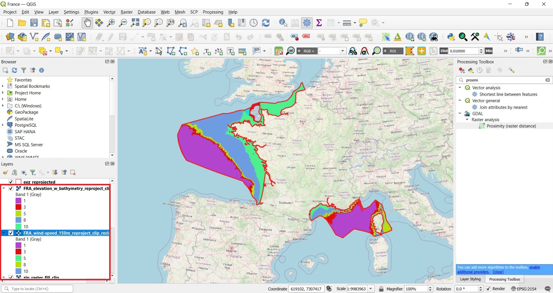
We are one step away from creating our final suitability map! Let’s combine the 3 rasters (bathymetry, wind and the Natura areas scores) by using ‘Raster’ on the main QGIS toolbar > ‘Raster Calculator’.

We will sum our raster files by multiplying each raster with the associated weight. This means that in the final Suitability Map, some criteria will ‘participate more’ on the solution and some other criteria less. Keep in mind that a raster file is a set of pixels! Thus, we are actually combine (sum) the score value of each pixel for every single criterion, for instance, (wind pixel score)*weight + (bathymetry pixel score)*weight + (Natura pixel score)*weight.

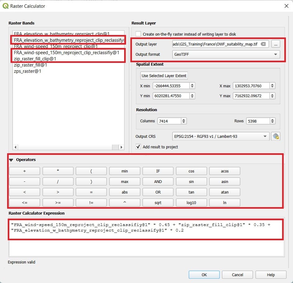
In ‘Raster Calculator’ (see the image above), we duble-click on each one of our criteria to insert the raster in the ‘Raster Calculator Expression’ and then we use the ‘Operators’ to do the multiplication of each criterion with the associated weight! Our formula should look like:

“FRA_wind-speed_150m_reproject_clip_reclassifiy@1” * 0.45 + “zip_raster_fill_clip@1” * 0.35 +
“FRA_elevation_w_bathymetry_reproject_clip_reclassify@1” * 0.2

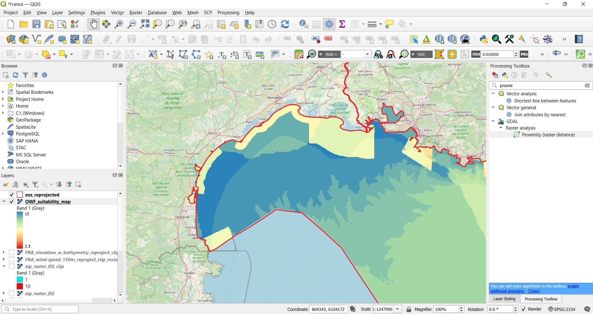
We save our ‘Result layer’ as ‘OWF_suitability_map! The result, after we change the ‘Symbology’ > ‘Singleband Pseudocolor’ > ‘Spectral’, will look like this…

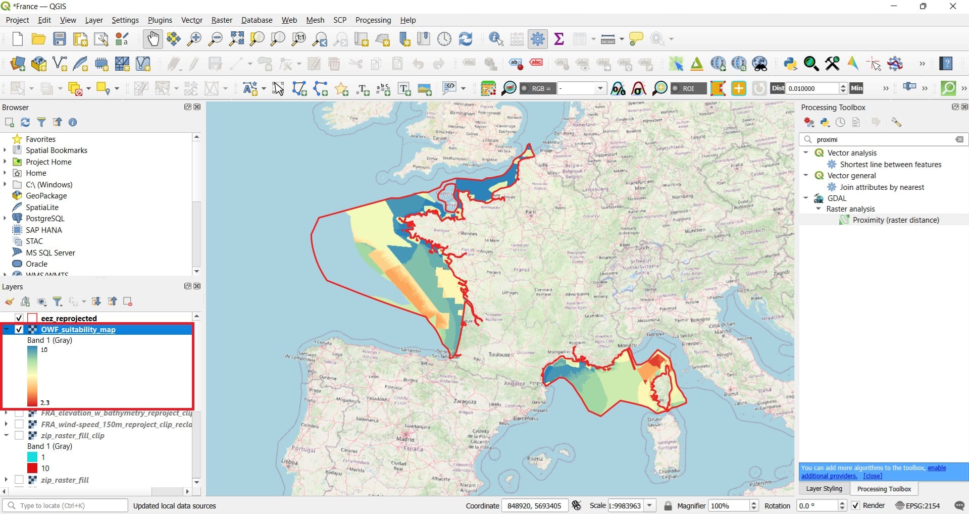
Blue areas indicate the best areas for placing our Offshore Wind Farm, yellow areas are less optimal and the red areas probably is not a good and viable solution to place our Wind Turbines. Hence, we see that there are plenty of optimal areas in the north-west coasts of France and in south-east coasts of the Mediterranean! This means that those areas have increased wind speeds AND low depth values AND they are not Natura areas! Also, the final scores range between 2.3 – 10. How is that possible? Why not between 1 – 30 since we summed 3 criteria and each criterion had a scale of 1-10? Don’t forget the weights we applied!

One pixel might has a score of 8 (wind), 9 (bathymetry) and 7 (Natura). If we sum those values without using weights, this equals to 24. But, if we apply the weighting scheme it’s (8*0.45)+(9*0.2+7*0.35) which equals to 7.85!

Let your students zoom in and explore different areas!

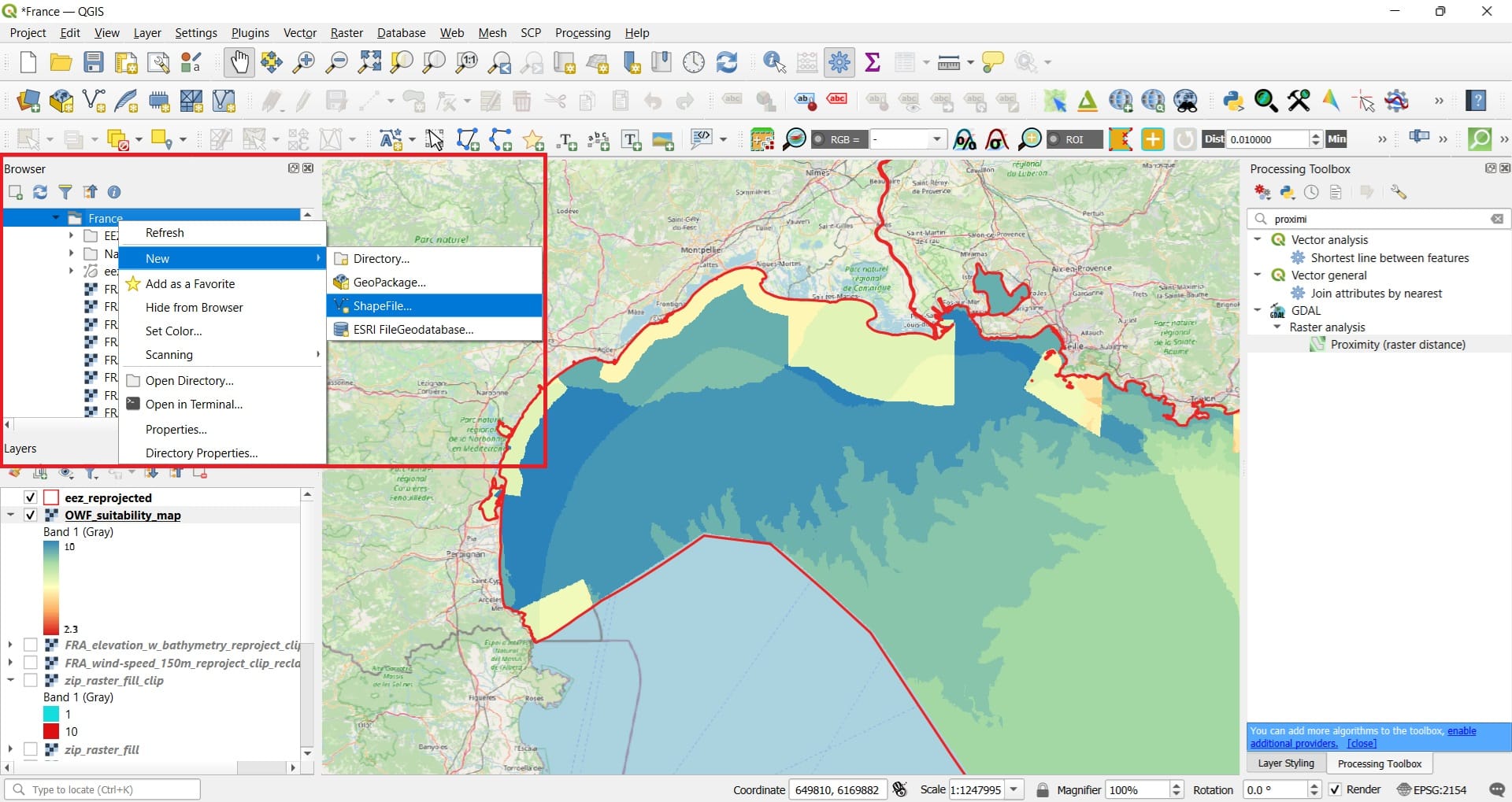
They may also create a new polygon shapefile and digitize their selected area (we saw that in the previous lessons!). Just navigate to the ‘Browser’ tab, find your folder > Right-click > New > Shapefile.

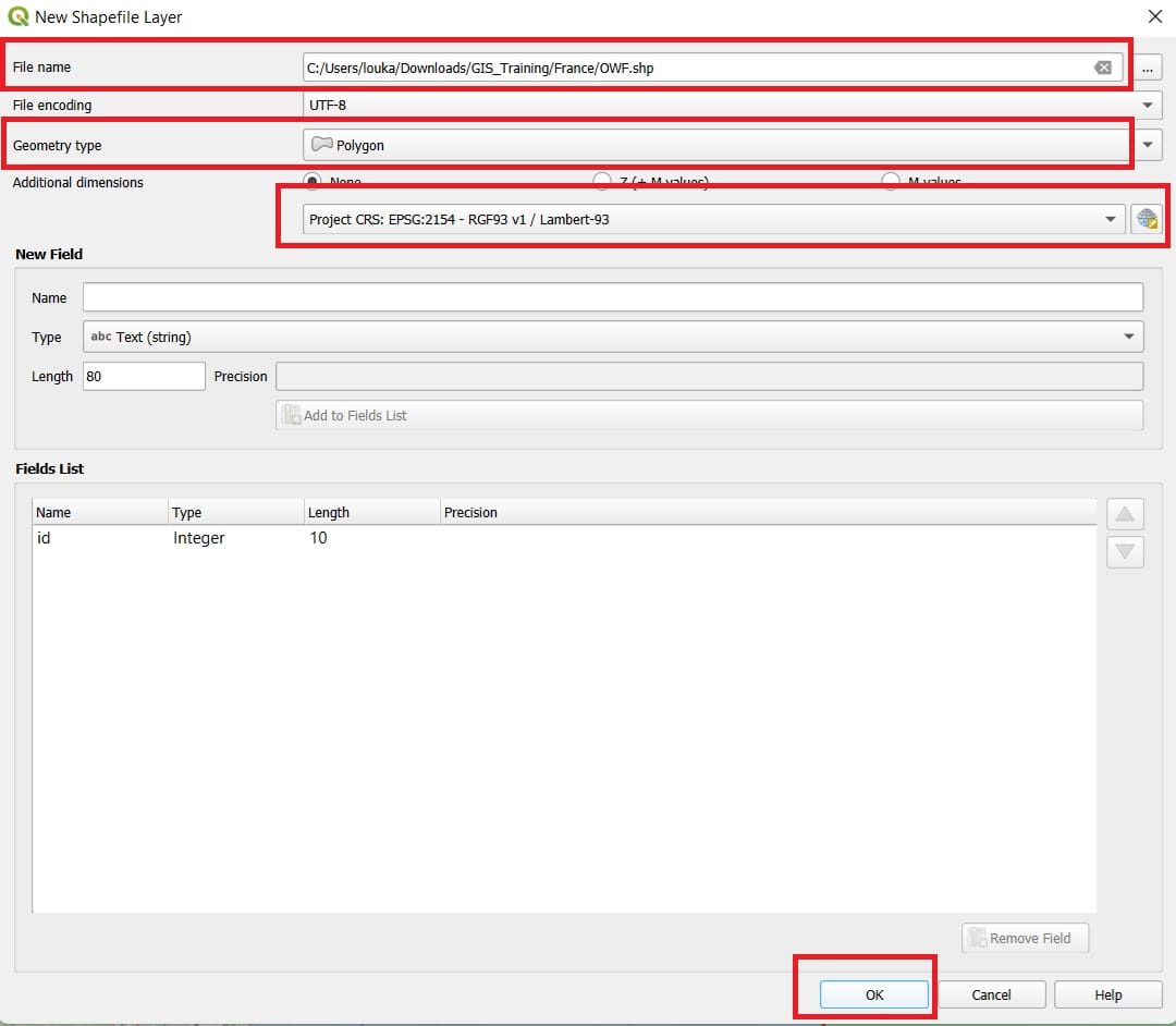
Name the new shapefile as ‘OWF’, select the type (Polygon) and set the appropriate CRS (EPSG: 2154)!

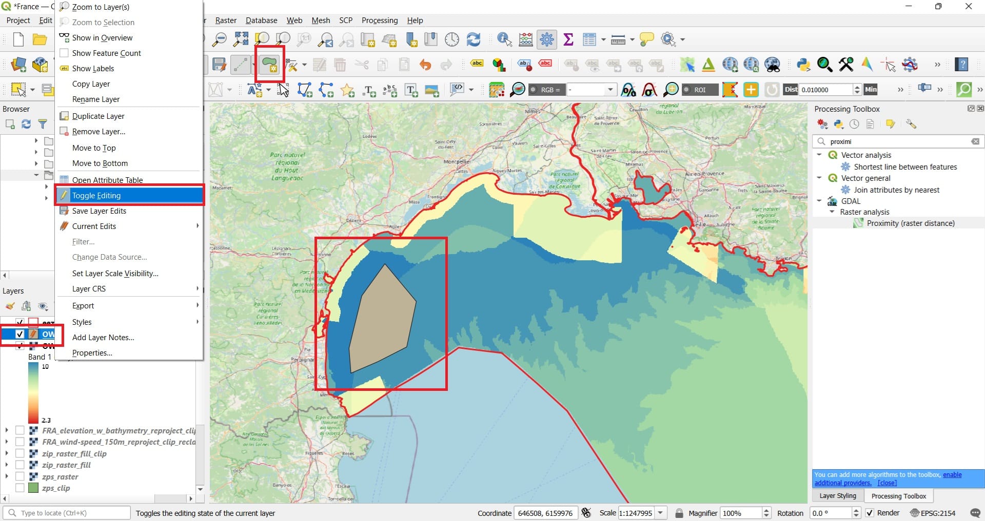
Load your new ‘OWF’ shapefile > Right-click on it > ‘Toggle Editing’ > Select the polygon digitization button on the main QGIS toolbar > Start editing your polygon and > after the last point right-click and add a value of 0 on the ‘id’ column! That was it!

Of course, if you think that this process we followed during the previous and the current lessons is complex, you may just use printed maps via the Global Wind Atlas and other Natura areas data portals (i.e. hereand here) and let your students explore the maps, read the legends, identify different wind and bathymetry patterns and combine the maps to identify the optimal areas!

During the next lesson, we will explore different processing capabilities and how we can create additional criteria for our projects like how to estimate the slopes of a surface, the aspect or even how we can interpolate point data information to create rasters!

Also, keep in mind that you may use Vector-based Multi-Criteria Analysis (MCA) which is particularly useful when working with discrete spatial features like parcels, buildings, or administrative boundaries. This approach leverages the attribute data associated with vector features, allowing for detailed analysis without the need to convert data into raster format. Take a look on the following videos!

In a nutshell, do not hesitate to identify different types of problems, data sources and overall, ideas to create project-based GIS activities for real-world problems! Keep always in mind that a multi-criteria problem like this is always based on an inquiry process, helping your students enhancing their critical and systems thinking as well as their problem solving skills, by simply using the following steps:

🧭 GIS-MCDA Steps – A Guide for Teachers

1. Define the learning problem or objective
Start by helping your students clearly state what they want to solve or explore. For example: “Where is the most suitable area for a new school garden?” or “Which parts of the city are most affected by air pollution?” or “Where to install some offshore wind turbines in France, Portugal, Greece etc.?”

✅ Encourage curiosity-driven or place-based questions. Show them maps and relevant information.
✅ Link the topic to the curriculum (e.g., geography, sustainability, STEM).

---

2. Choose criteria and identify any constraints
Guide students in selecting the factors (criteria) that will help them solve the problem, and any limitations (constraints) that must be considered. These could come from their own ideas, classroom discussions, or simple research.

✅ Use maps, online resources, or interviews to support selection.
✅ Encourage critical thinking: What matters? What gets in the way?

---

3. Transform the values into a common scale
Since each layer may have different units (e.g., wind speed, distance, land type), help students understand the need to standardize the data—so they can be compared fairly.

✅ Use simple scales like 1–5 or 1–10 for classroom use.
✅ You can do this in QGIS using raster reclassification tools or the conversion to raster tools we explored.

---

4. Assign weights to the criteria
Some criteria are more important than others. Have your students decide how much each factor should count toward the final decision. This encourages discussion and collaborative decision-making.

✅ Use methods like class voting or pairwise comparisons.
✅ Explain that weighting reflects values and priorities.

---

5. Combine all the layers
Now it’s time to bring all the information together! QGIS allows you to combine layers mathematically to create a composite map that shows the most suitable areas.

✅ Use the raster calculator to add weighted layers together.
✅ The output will visualize the “best” zones based on students’ choices.

---

6. Review and reflect on the results
Ask students to analyze the final map and reflect: Does the result make sense? Would it change if we adjusted a criterion? This step builds critical thinking and shows that spatial analysis involves choices and trade-offs.

✅ Encourage “what if” discussions or simple sensitivity analysis.
✅ Invite students to present and justify their decisions.

Wrapping Up: Multi-Criteria Problem-Solving in GIS

Congratulations on completing the Multi-Criteria Problem-Solving lesson! In this course, you’ve learned how to move from basic spatial data processing to building meaningful, real-world decision models using GIS and raster analysis.

You started by preparing and processing raster layers—clipping, reclassifying, and converting data into forms that can be analyzed together. These steps weren’t just technical exercises—they were essential to set the stage for the next level of spatial thinking. Then, we introduced you to the concept of Multi-Criteria Decision Analysis (MCDA)—a structured way to evaluate multiple factors in a spatial context. You learned how to:

✅ Define a spatial problem or objective (e.g. siting offshore wind farms)
✅ Select relevant criteria and constraints using informed discussions and data sources
✅ Standardize the input data so that different layers can be compared
✅ Assign weights to each criterion based on their importance—whether using simple classroom judgment or more formal methods like AHP
✅ Perform a weighted overlay to combine layers into a single suitability map

Most importantly, you’ve seen how this kind of analysis can be made accessible and engaging for students—building not only GIS skills, but also critical thinking, collaborative decision-making, and spatial literacy.

🧭 Ready for more? In the next course, we’ll take these skills even further—exploring surface analysis and 3D objects, advanced analysis in GIS.

Well done—and keep thinking spatially! 🌍📊🗺️

Useful links

1. Malczewski J., (2006). GIS-Based Multicriteria Decision Analysis: A Survey of the Literature. International Journal of Geographical Information Science: 20(7);703-726.
2. Malczewski, J., and Rinner, C. (2015). Multicriteria Decision Analysis in Geographic Information Science. Springer.
3. Darwish, K. (2023). GIS-Based Multi-Criteria Decision Analysis for Flash Flood Hazard and Risk Assessment: A Case Study of the Eastern Minya Watershed, Egypt. Environmental Sciences Proceedings, 25(1), 87.
4. Gigović, L., Drobnjak, S., & Pamučar, D. (2019). The Application of the Hybrid GIS Spatial Multi-Criteria Decision Analysis Best–Worst Methodology for Landslide Susceptibility Mapping. ISPRS International Journal of Geo-Information, 8(2), 79.
5. Ifkirne, M., El Bouhi, H., Acharki, S., Pham, Q. B., Farah, A., & Linh, N. T. T. (2022). Multi-Criteria GIS-Based Analysis for Mapping Suitable Sites for Onshore Wind Farms in Southeast France. Land, 11(10), 1839.
6. Saaty R.W. (1987). The analytic hierarchy process—what it is and how it is used, Mathematical Modelling: 9(3-5); 161-176.
7. WindEdition: Introducing Different Types of Offshore Wind Turbine Foundations: Fixed and Floating