Creating 3D surfaces

🏔️ Creating 3D Surfaces in QGIS

In this lesson, we take your GIS skills to the next dimension—literally! You’ll learn how to create and visualize 3D surfaces using Digital Elevation Models (DEMs) and QGIS plugins. By bringing elevation and terrain data to life, students can gain a much deeper spatial understanding of landscapes, topography, and environmental variables.

Working with 3D surfaces is not only useful in geography and Earth sciences—it’s also a powerful tool for urban planning, hazard mapping, landscape design, and climate studies. It adds depth and realism to your spatial analysis, making your projects more engaging and insightful.

✅ What You’ll Learn

✅ Understand different types and applications of 3D modelling
✅ Learn how to load and prepare elevation data in QGIS
✅ Use QGIS plugins to create and manipulate 3D surfaces
✅ Explore how 3D visualizations enhance analysis and communication
✅ Apply these skills to create your own 3D terrain models in the classroom

By the end of this lesson, you’ll be able to transform flat maps into detailed landscapes and mountains, helping students visualize their world in three dimensions. Let’s get started and see what your terrain looks like in 3D! 🌍⛰️🧱

🌍 GIS and 3D modelling

Most maps are two dimensional, and two-dimensional maps will always be useful. However, many real-world features, such as wells, underground transportation lines, flight paths, elevator shafts in a building, and subsurface geological formations, have more meaning when visualized in 3D. In this course, you will learn about the types of data that are used to model the real world in 3D scenes, including functional surfaces and 3D feature types [1].

3D representation capabilities

In modern GIS, working in three dimensions allows us to model and visualize the world in rich detail, whether we’re mapping terrain, underground structures, or urban infrastructure. With 3D GIS, we can represent complex features such as:

3D point clouds as sample points collected in the air or below ground
3D linear entities like literally space curvesfor example, boreholes or power lines in industrial plants.
3D non-planar surfaces, which may be smooth, continuous, fragmented, or irregular.
3D solids with regular geometries, such as tunnels, wells, or infrastructure.
3D irregular solids—like clouds, ore bodies, or pollution plumes, that have variable interior properties and may be continuous or disjointed.

Understanding these different 3D elements expands our analytical capabilities in GIS, from urban planning to environmental monitoring and complex spatial modeling.

Common 3D applications

There is a variety of applications using 3D geodata in different fields, such as geoscientific appplications (geology, mining, oceanography) , environmental monitoring , hydrology, infrastructure networks, cadaster, urban planning, smart cities, archaeology, computer games, education, etc. Commercial systems (ESRI, Hexagon Geospatial, Geoweb 3d, GRASS GIS, GeoScene3D, etc.) offer integrated, general or specialized 3D capabilities for analysis and visuaization – something impossible in the older days. In this section, a number of exemplary 3D applications are presented, starting from geoscientific ones and then moving towards more unusual ones.

Geology: A linear representation of mine excavations (tunnels, shafts, ramps, bore-holes) using 3D space curves

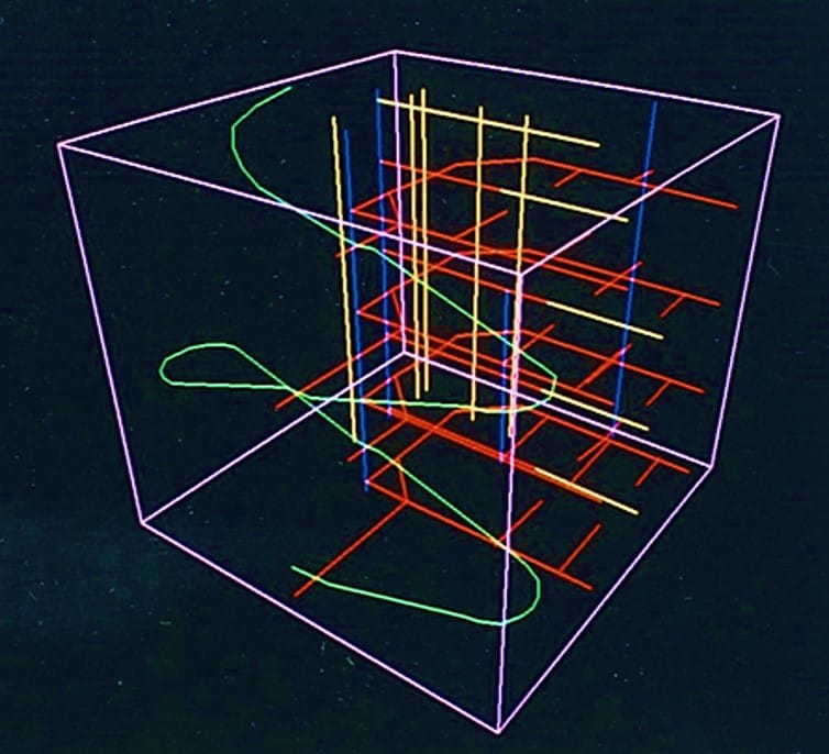
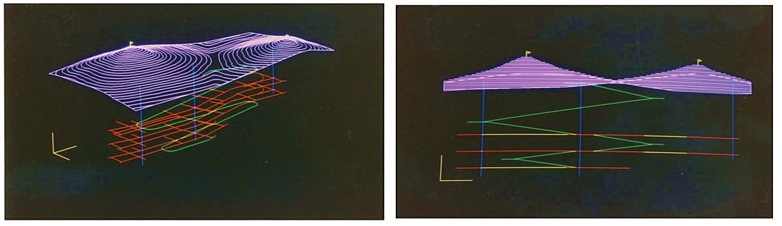
Geology: A linear/wireframe representation of surface 2.5D topography and underground mine excavations (tunnels, shafts, ramps, bore-holes) using 3D space curves

Urban environment: (a) Aerial axonometric view and (b) 3D representation of the Sant Andreu District of Barcelona – license CC BY 4.0.

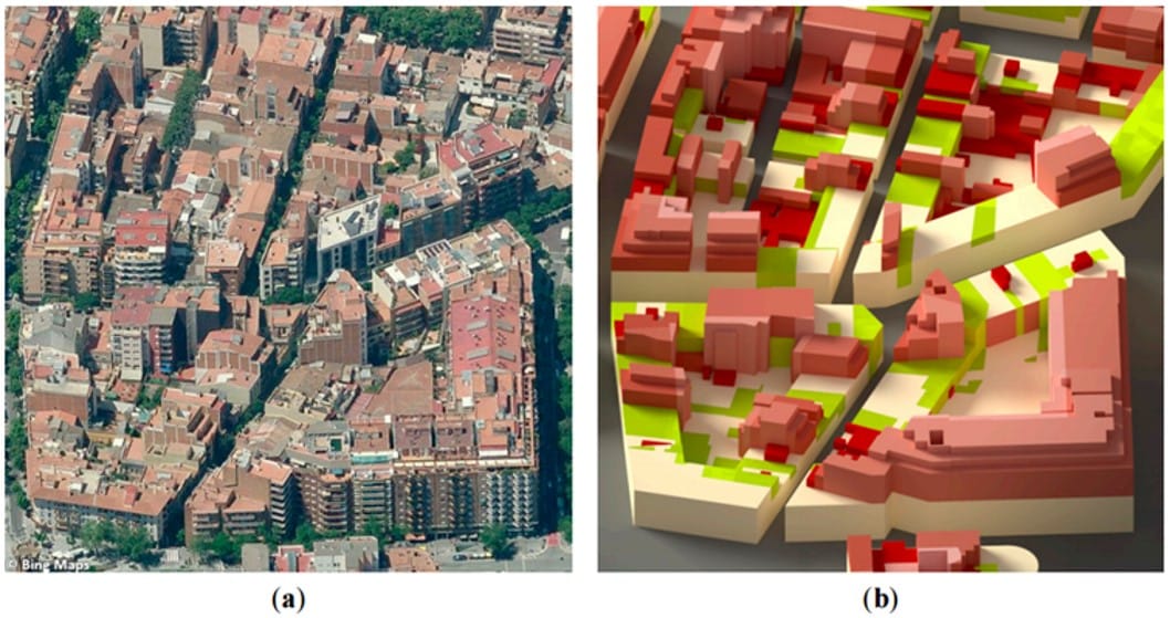
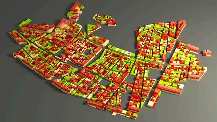
Urban environment: Volumetric analysis of built-up area of the Sant Andreu District of Barcelona – license CC BY 4.0.

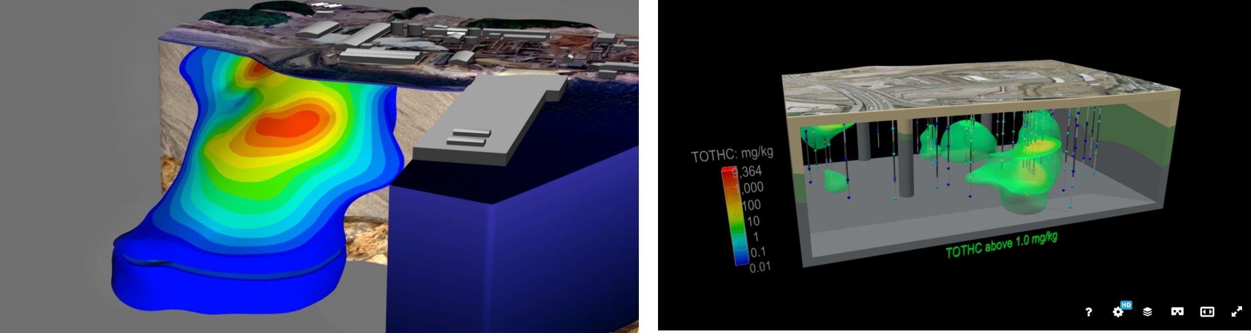
Environmental Modelling: The Use of 3D Modelling for Environmental Site Assessment

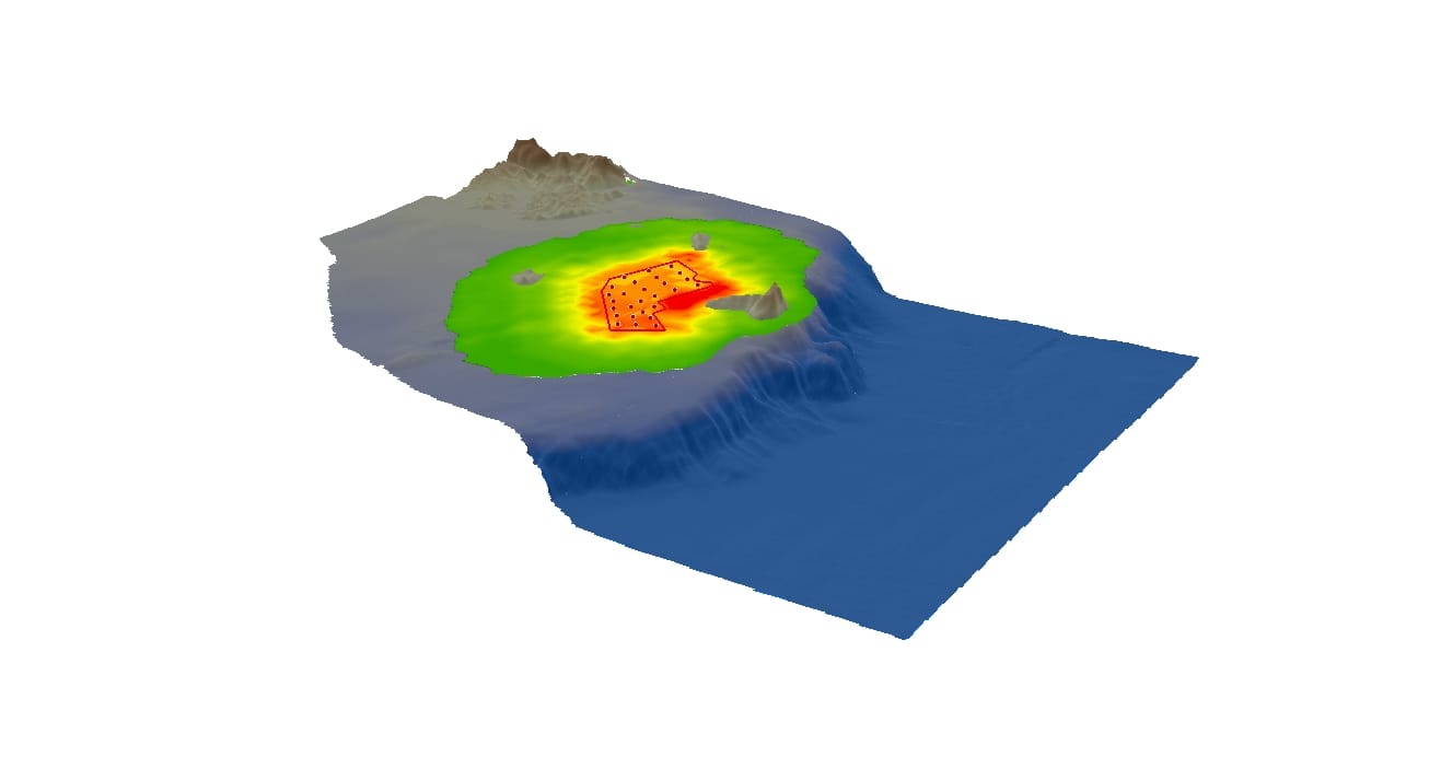
Topography and environmental modelling: The Use of 3D Modelling for visualizing sea topography and environmental impact from offshore wind farms

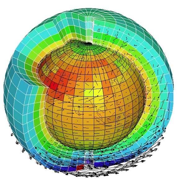
Environmental modelling: Weather forecasting applications, Image Source: Encyclopedia of the environment

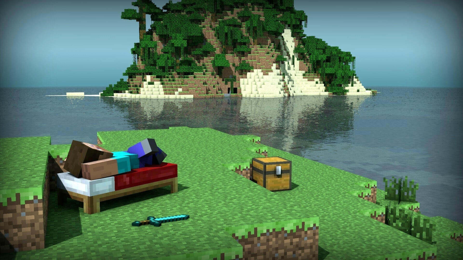
Gaming: GIS mapping in video games means gamers can experience precise terrains, climates, infrastructures, and more since games that utilize these technologies. Developers on projects such as Call of Duty, Grand Theft Auto, Far Cry, and SimCity have also been able to replicate topography, land use patterns, and climate data into these games and series. Image Source: All3DP

🌍 Creating our own 3D model using QGIS

Let’s try to create our own 3D visualizations using QGIS. First we open QGIS and we create a new project! We should also save it as ‘Sweden’ because this time, we travelo to Sweden!

You may save your project in ‘GIS_Training’ folder by creating a new folder ‘Sweden’ for saving the data we will download.

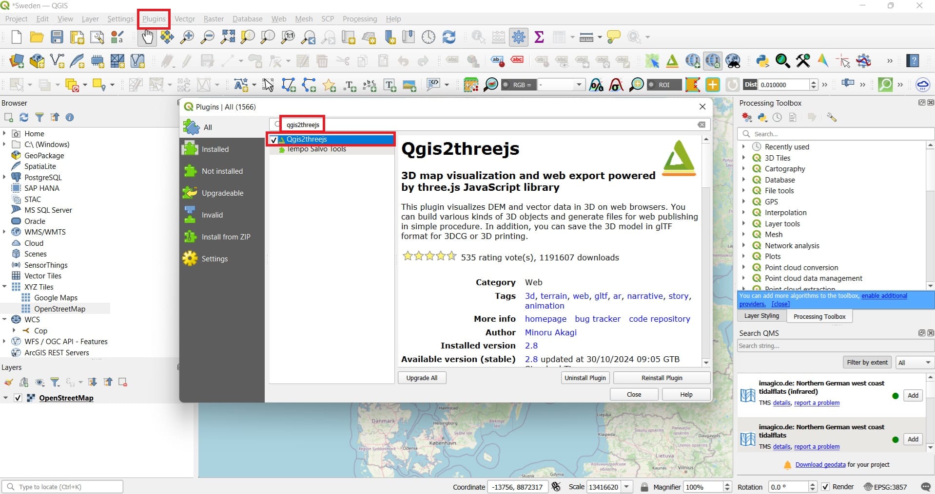
Next, we have to install the QGIS 3D plugin ‘qgis2threejs’. To do that, we select ‘Plugins’ in the main QGIS Toolbar > ‘Manage and install plugins’. You can type ‘qgis2threejs’ and install the plugin.

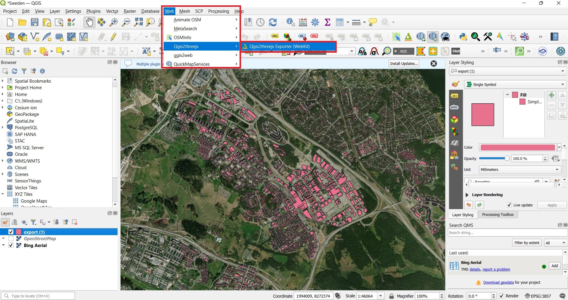
After you install the plugin, you may find it in the main QGIS Toolbar > ‘Web’ > ‘Qgis2threejs’ > ‘Qgis2threejs Exporter’.

Before we load the plugin and start experimenting, let’s download some data for Sweden! This time, we will use DivaGIS portal to download the Digital Elevation Model (DEM) for Sweden.

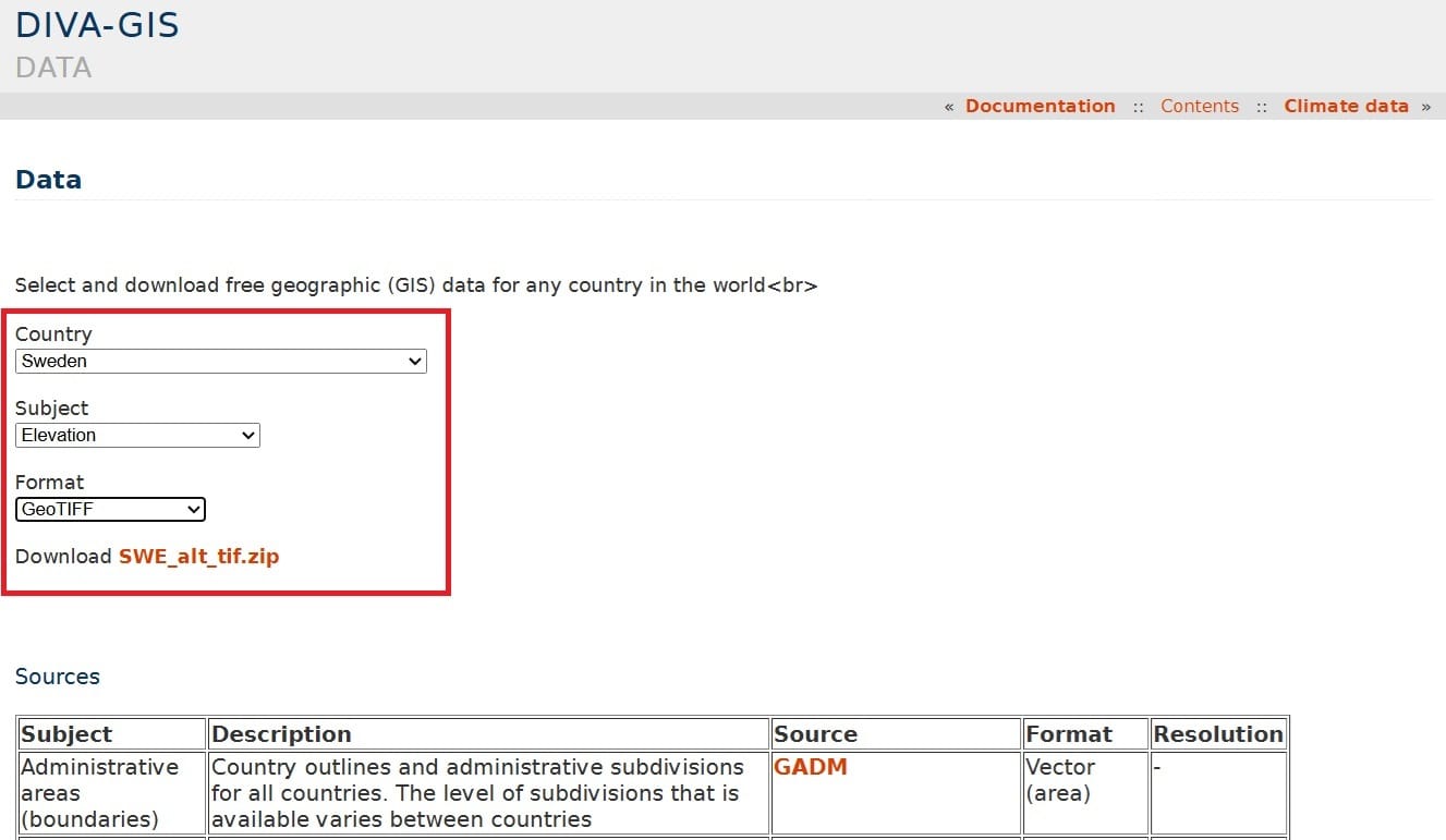
We select the country (Sweden), the subject (Elevation) and the format (GeoTIFF) and we press ‘Download’. We copy and extract our data to the ‘GIS_Training’ folder in the sub-folder Sweden.

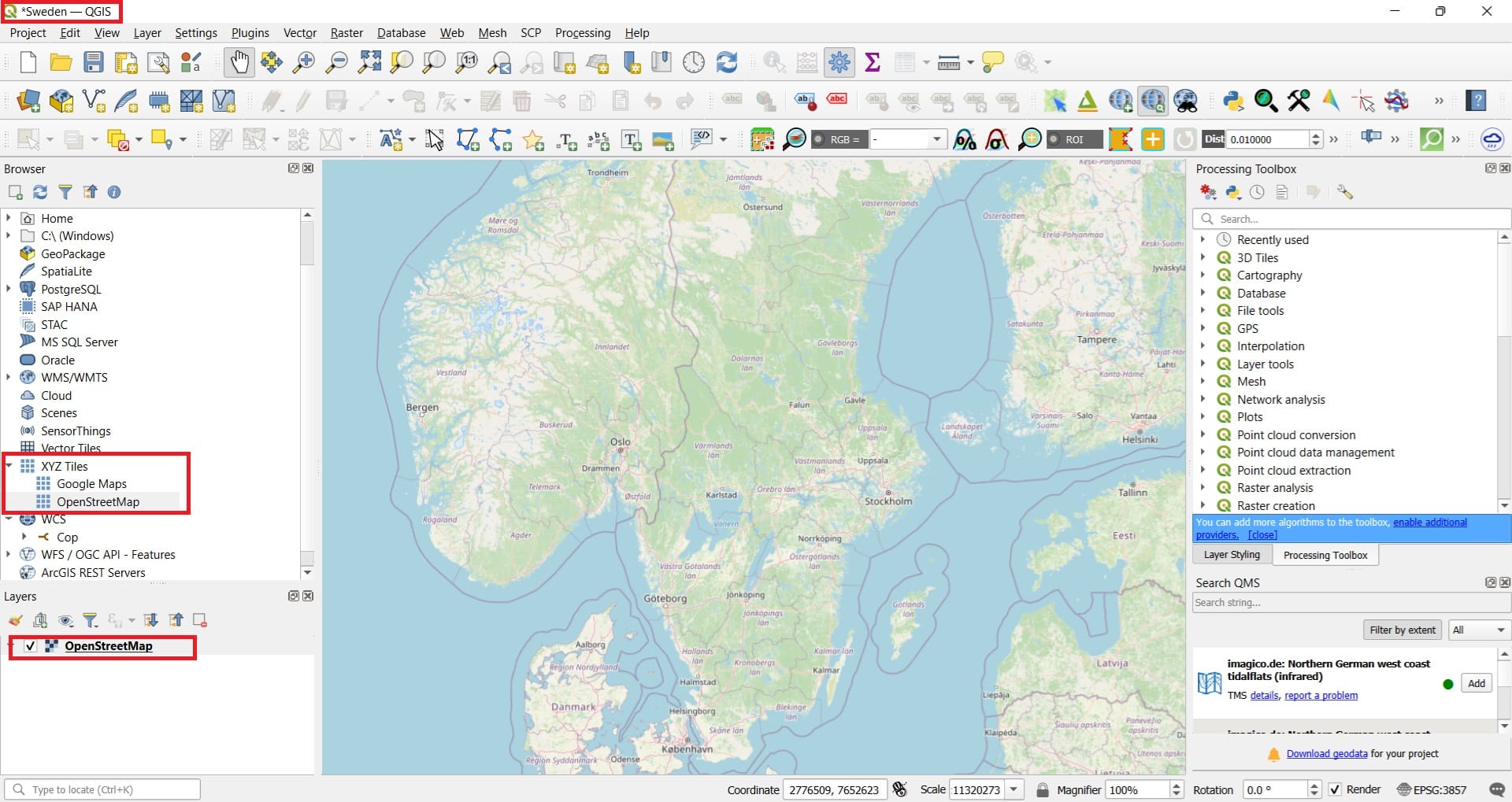
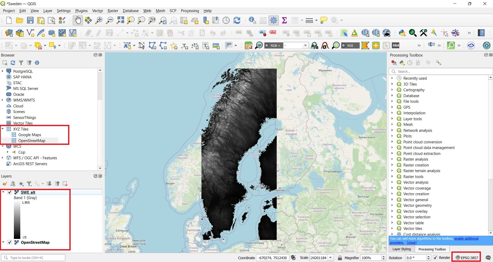
We load the ‘SWE_alt’ raster in QGIS and the Open Street Maps (OSM) basemap. IMPORTANT: Change the Coordinate Reference System (CRS) of the project from the geographic one, EPSG: 4326 (WGS 84) to the projected one, EPSG: 3857 (WGS 84 Pseudo-Mercator) at the bottom-right corner of QGIS (see the image below).

You may also change the ‘Symbology’ of your layer from black and white color scale to ‘Turbo’ by double-clicking on your layer > ‘Symbology’ > ‘Render type: Singleband Pseudocolor’ > ‘Color ramp: Turbo’.

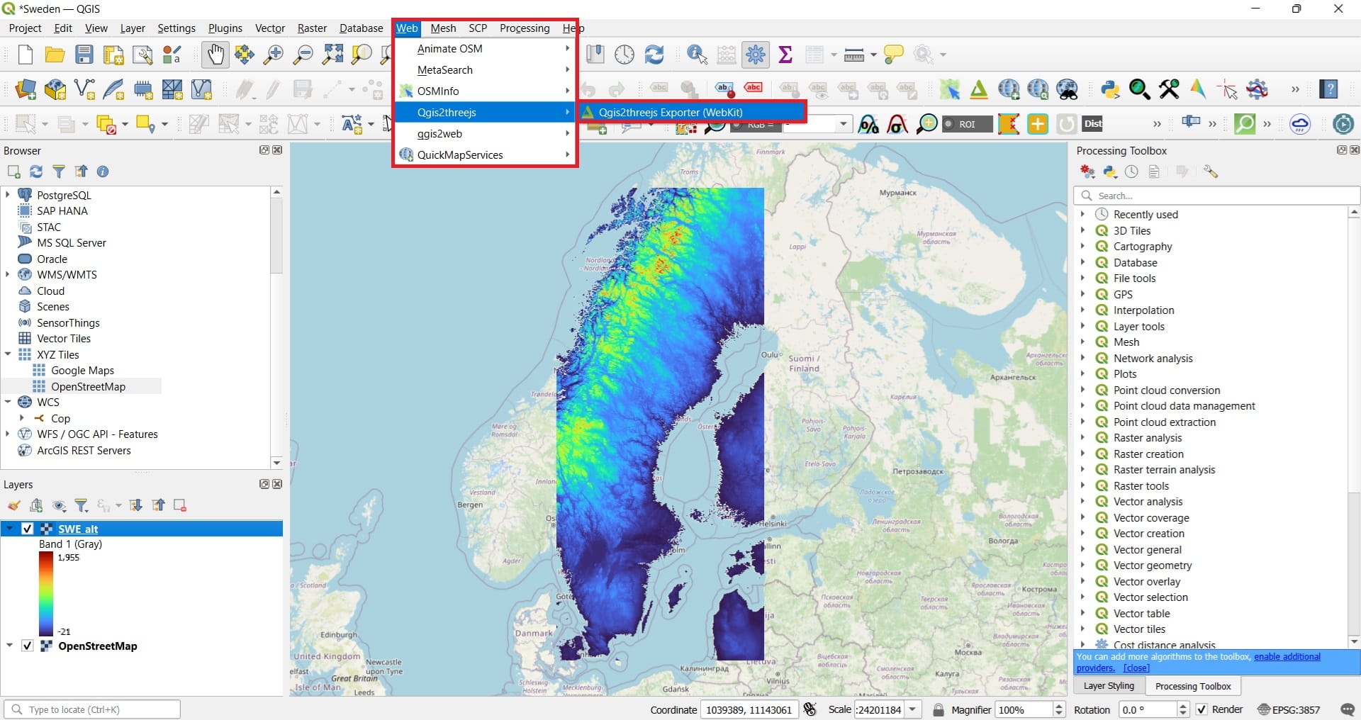
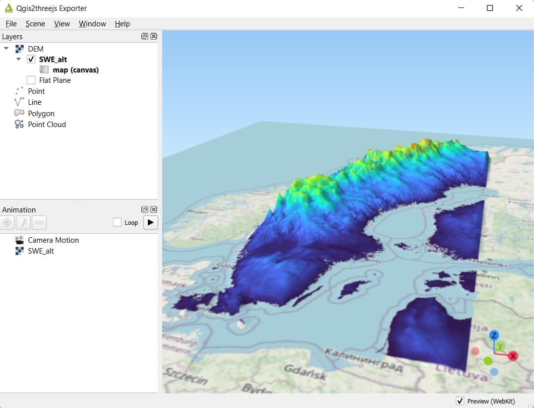
Next step is to open the ‘qgis2threejs’ plugin. To do that, we select ‘Web; on the QGIS main toolbar > ‘Qgis2threejs’ > ‘Qgis2threejs Exporter’.

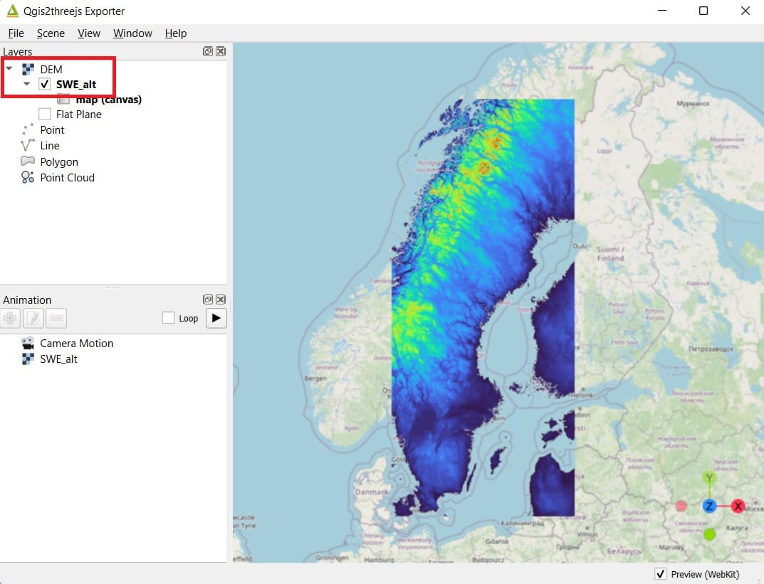
If you don’t see anything and the map window is blank, don’t worry. Just zoom-in!!! If you left-click on the map window you may rotate and change the 3D map orientation.

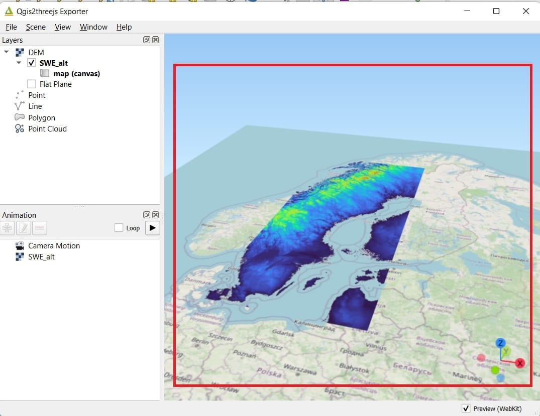
Does it look like 3D? Not yet…Why? Because we should change the Z factor exaggeration. In GIS, the Z factor is a scaling factor used to convert elevation values when they differ from horizontal (x,y) coordinate units, or to exaggerate the vertical dimension for visualization purposes. Essentially, it allows you to adjust how much the elevation values are stretched or compressed in a 3D representation.

In countries with high-elevation areas (i.e. Nepal), even with a Z factor of 0 or 1, you may be able to see the elevation difference quite easily. However, let’s be honest, Sweden is not a country with high-elevation mountains (maximum elevation value = 2000 meters), so, let’s try to stretch the elevation values in order to produce a better 3D result.

To do that, we select ‘Scene’ > ‘Scene Settings’ > ‘Z exaggeration’ = 200.

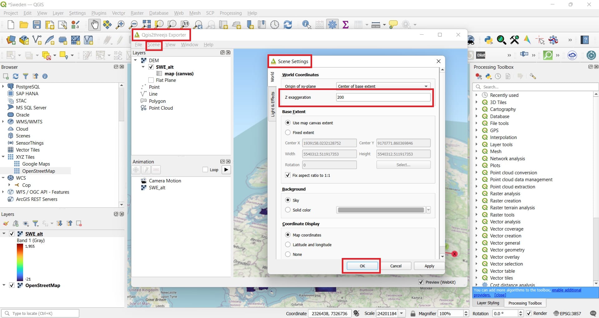
When we press ‘OK’, the result becomes a bit more interesting! You may zoom-in or zoom-out and by right-clicking and holding on the map window you may re-position the map.

By pressing on the ‘File’ button, you have 2 options, either to save your 3D visualization as an image or to save your 3D as an .html (web link).

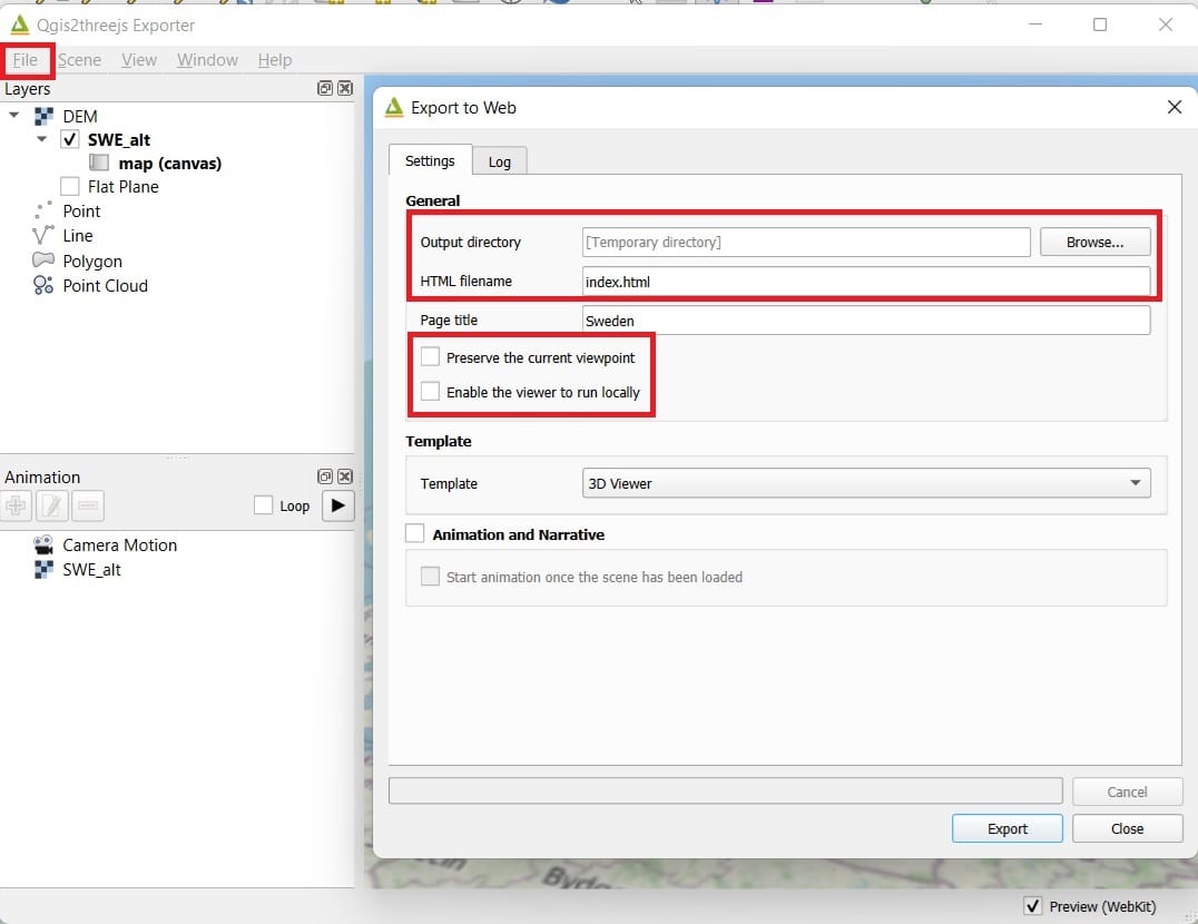
You select the folder to store your .html file and the files created by ‘Qgis2threejs’ for loading the web 3D file. If you want to share your maps with other users, you should add ALL THESE FILES to a folder, compress them and share them via email. Don’t forget to activate the ‘Checkboxes’ (see the image above) to preserve the current viewpoint you selected and enable the viewer to run locally!

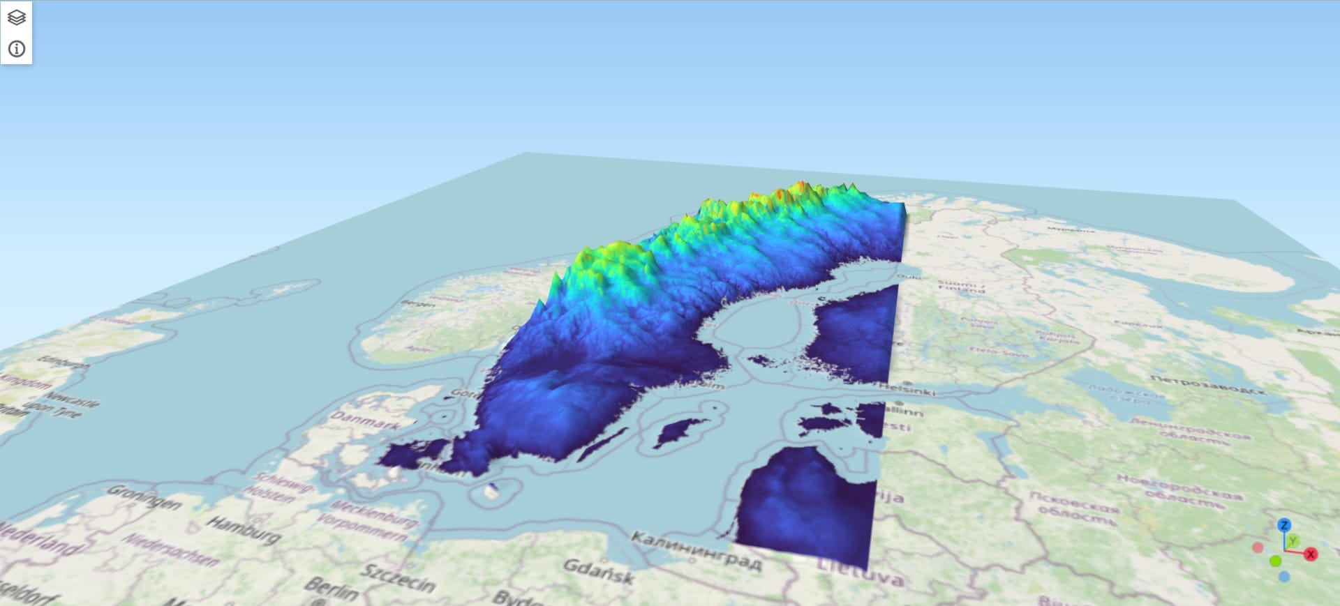
If you open the index.html file, the result will look to your browser like this:

Can we make it more impressive? Of course we can! Let’s try to add some buildings! This time we are not going to use BBike for downloading Open Street Map (OSM) vector data. Instead, we will use an amazing tool called Overpass API! Why? Because we want to download some buildings in Stocholm, including the buildings heights or levels/floors and BBike can’t do that.

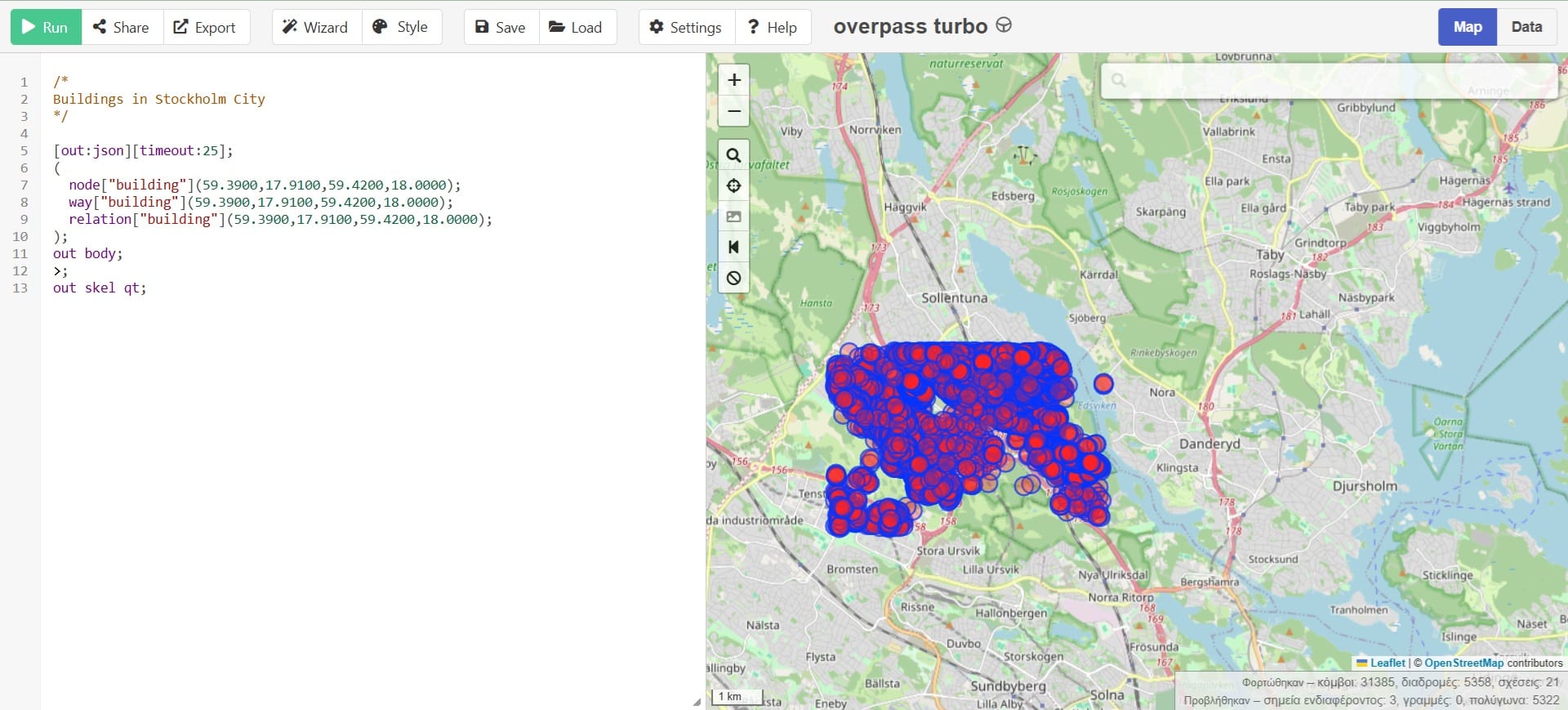
In the image above, you may see the Overpass API browser. It looks complex but, it’s not that much. The only thing we need to know is the code and the bounding box (bbox) coordinates of the area we want to download data.

The code you need to copy and paste is:

/*
Buildings in Stockholm City
*/

[out:json][timeout:25];
(
node[“building”](59.3900,17.9100,59.4200,18.0000);
way[“building”](59.3900,17.9100,59.4200,18.0000);
relation[“building”](59.3900,17.9100,59.4200,18.0000);
);
out body;
>;
out skel qt;

The bounding box coordinates for your city can be extracted by BBox Finder (link):

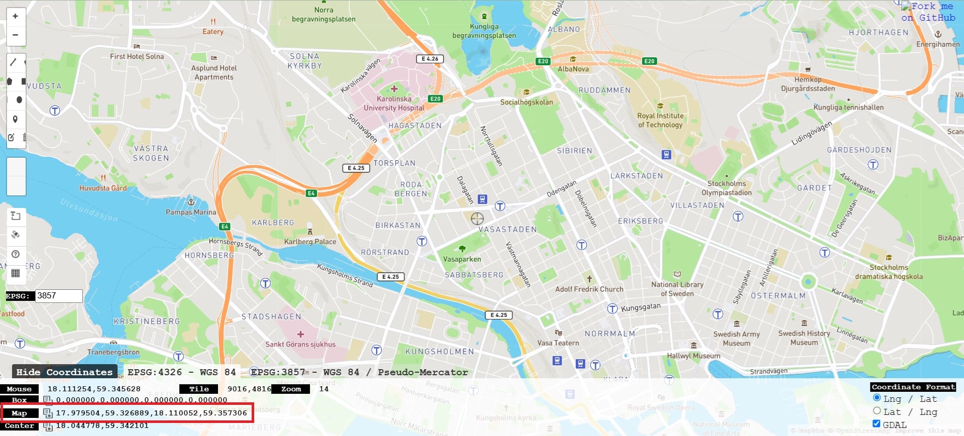
Thus, the only thing you need to do is to copy and paste the code and just change the min-max latitude and longitude and latitude coordinates!

Then, you press ‘RUN’ and ‘EXPORT’ as geojson file. Now you can load it as a shapefile layer in QGIS!

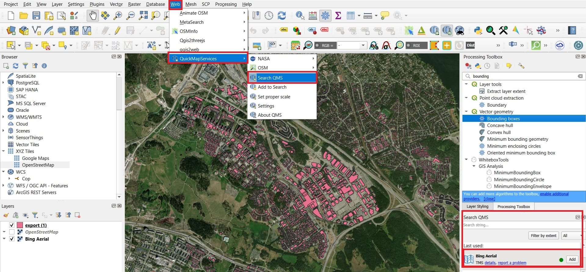
In QGIS, instead of the Open Street Map (OSM) basemap, you can load the Bing Aerial (Satellite) basemap! To do that, you select ‘Web’ on the main QGIS Toolbar > ‘QuickMapServices’ > ‘Search OMS’ and on the bottom-right corner of QGIS you ‘Search’ for ‘satellite’ and you click ‘Add’ on ‘Bing Aerial’ or ‘Bing Satellite’.

You also load the buildings geojson file (export.geojson) you have downloaded (see the image below).

Now we are almost ready to cready our buildings 3D scene! However, we must identify and adjust the buildings heights in the Attribute Table!

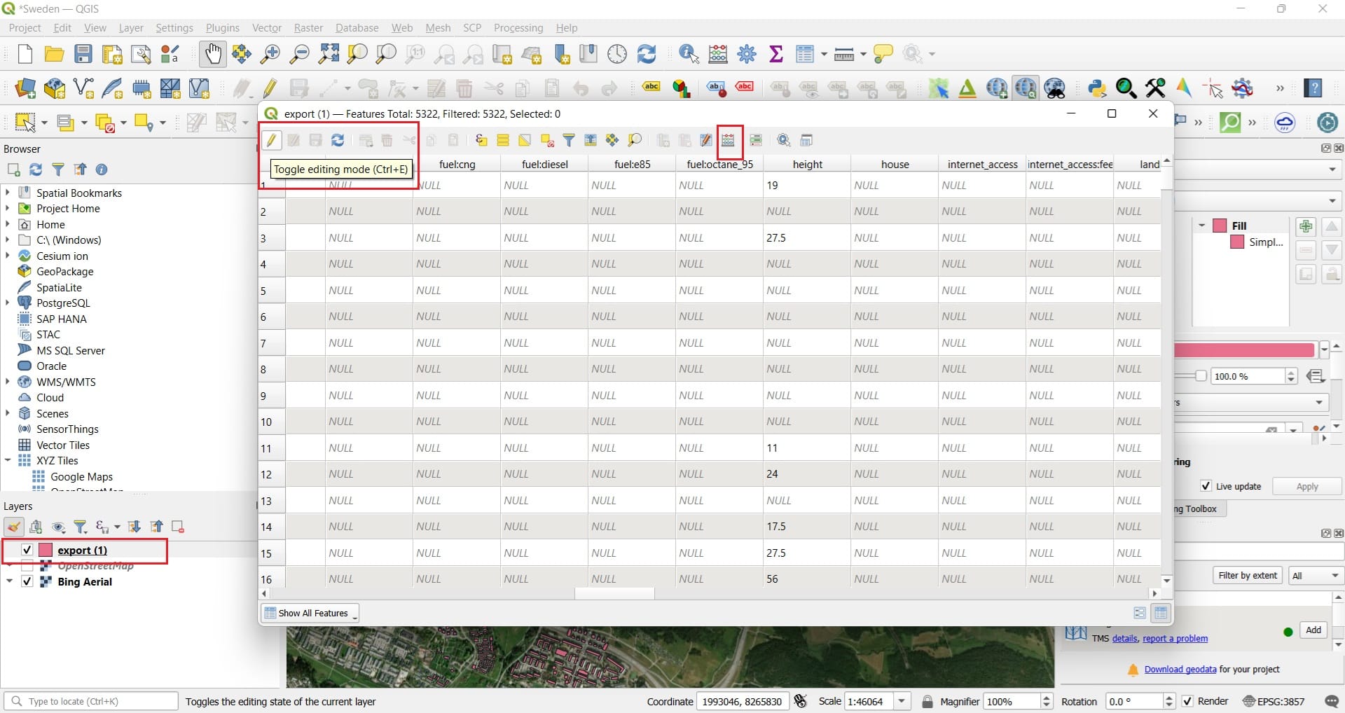
In the ‘Attribute Table’, we first select ‘Toggle editing mode’ (first icon) and then the ‘Filed Calculator’ (see the image above). Why are we doing this? Because we want to calculate the height of the buildings to create our 3D visualization. The ‘export.geojson’ Attribute Table includes the height of the buildings (height field) and the buildings:levels (levels, i.e. no. of floors) information. However, the numbers you see are not numbers but text!

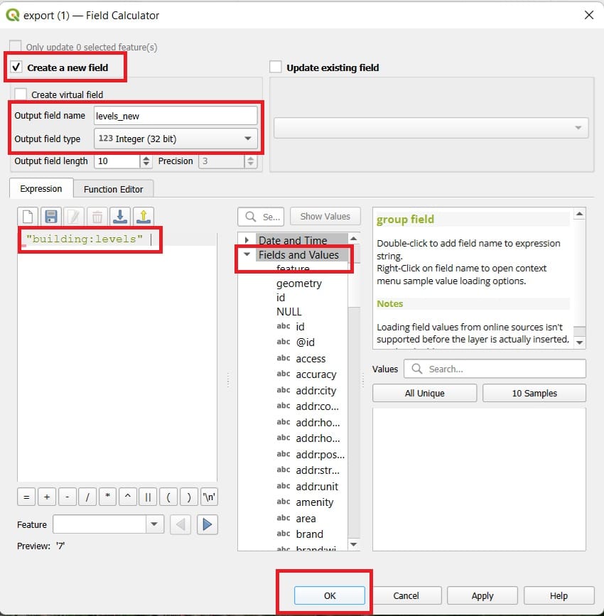
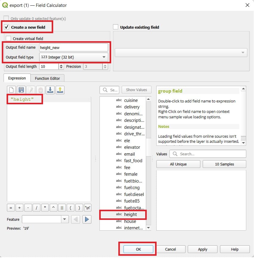
If we want to perform some calculations, we should trnasform both fields to numeric values and to do that, we will create 2 new fields, ‘height_new’ and ‘levels_new’! Hence, in the ‘Field Calculator’ window we select > ‘Create a new field’ > ‘name: levels_new > field type: Integer (32 bit) and in the expression window we type ”building:levels”.

Instead of typing the ”building:levels” in the expression window, you may double-click the third buildings field in the ‘Fields and Values’ list which includes all the attributes listed in the Attribute Table. Then, you press ‘OK’.

We repeat the same process for the ‘heights_new’ field!!!

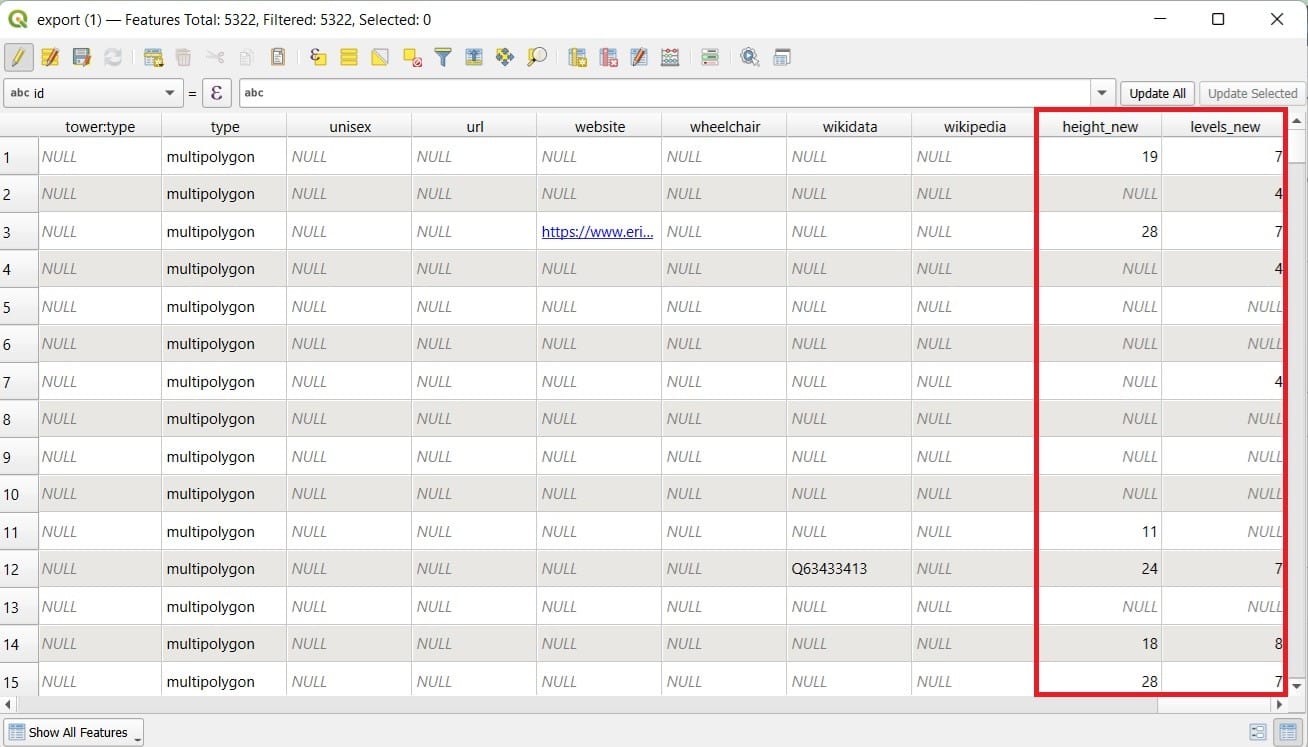
Now that we have the new fields, we want to calculate the buidlings heights for as many buildings as we can! To do that, we will multiply the levels per building with a value of 4 (in meters), considering that each building floor has a height of 4 meters. Ok, 4 meters might be too much but, we want to create something slightly more impressive with our students.

For the buildings we have the height value, we don’t change anything. For some buildings though, we only have the ‘levels’ value. Using ‘Field Calculator’ again, we will create a new expression in the form of:

If the ‘height_new’ value is NULL (empty), then extract each building height by multiplying the number of levels by 4 (levels_new*4), otherwise (if the height_new has a value), keep the building height current value. The exact expression is:

if( “height_new” IS NULL, “levels_new” *4, “height_new” )

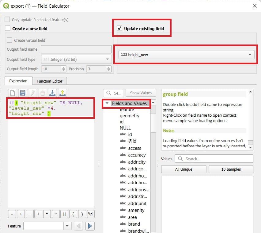
Let’s open again the ‘Field Calculator’ in the Attribute Table’!

This time we are not creating a new field but we are updating an existing one, the ‘height_new’ field. Select > ‘Update existing field’ > ‘height_new’ > write the expression in the ‘Expression’ window:

if(“height_new” IS NULL, “levels_new” *4, “height_new” )

We press ‘OK’.

IMPORTANT! Be sure that you gave the exact same names in the new fields otherwise, feel free to write the expression from scratch and select the field names by double-clicking on the ‘Fields and Values’ list.

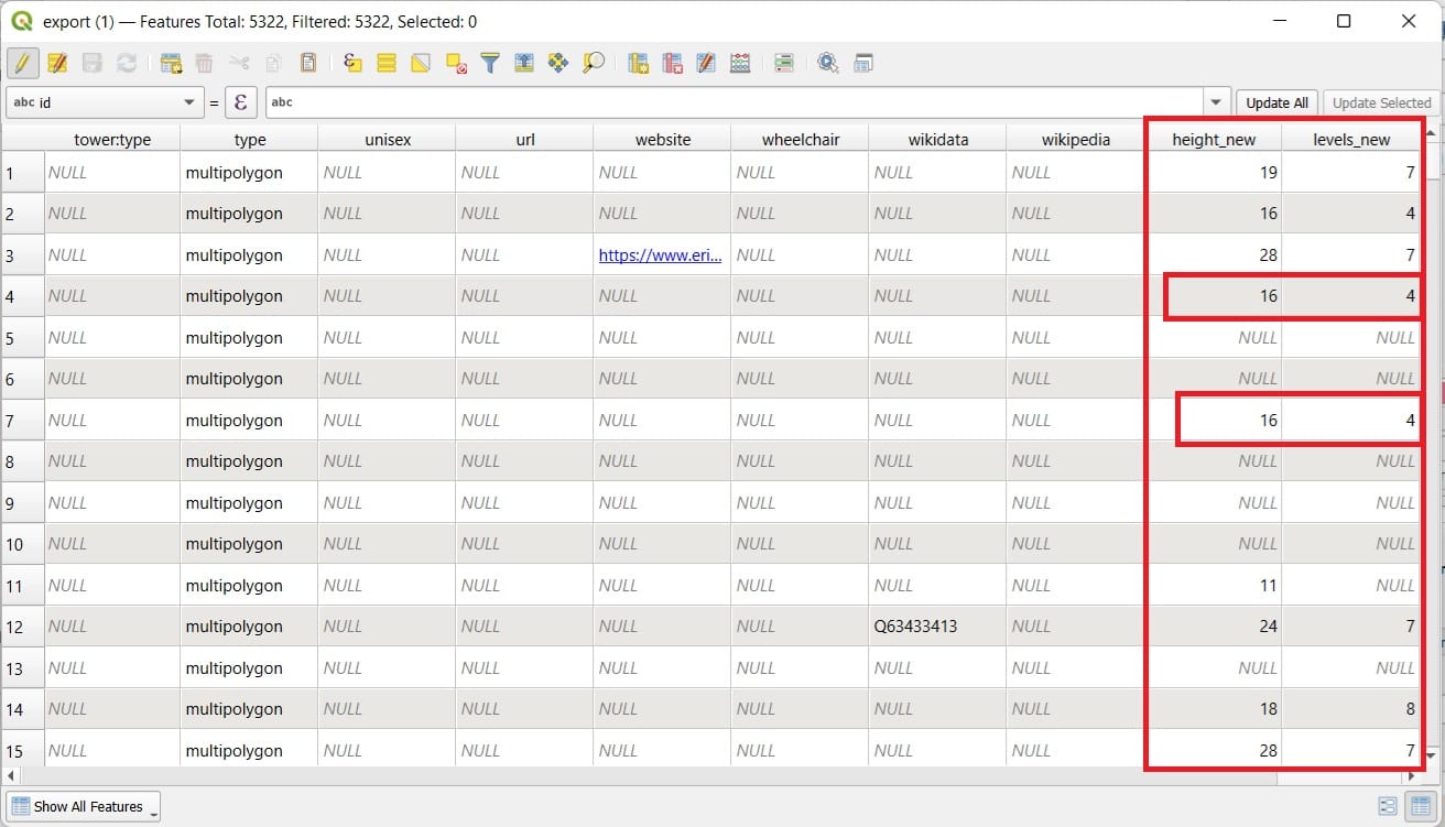
As you can see in the updated table below, some height values have been updated!

Let’s create our new 3D visualization! We select ‘Web’ on the main QGIS toolbar > ‘Qgis2threejs’ > ‘Qgis2threejs Exporter’.

MAKE SURE THAT THE SELECTED EPSG IS ‘3857’ (WGS 84 World Mercator) IN THE BOTTOM-RIGHT CORNER OF QGIS!

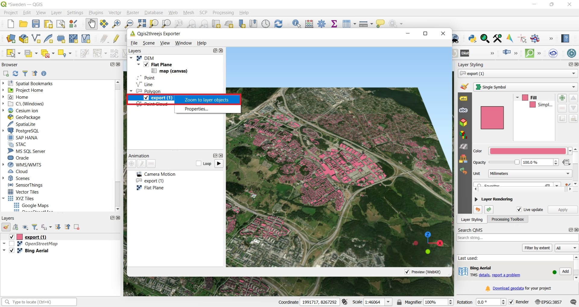
When you open Qgis2threejs, if you don’t see the map or it looks far far away, just righ-click on the ‘export’ file and select ‘Zoom to layer objects’. Also, make sure that the Satellite Basemap is activated on the QGIS Layers Tab.

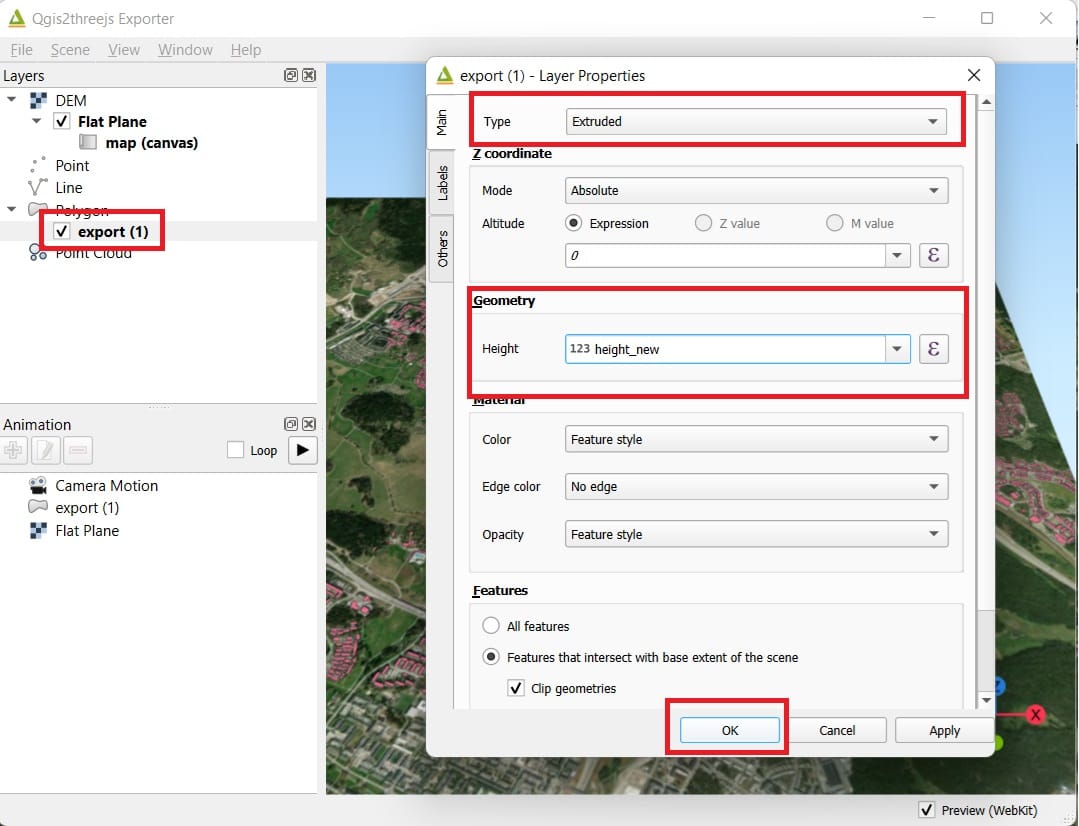
We are 2 moves away from creating our 3D! First, we double-click on the ‘export’ file and we select (see the image below):

Type: Extruded
Geometry > Height: height_new
We press ‘OK’

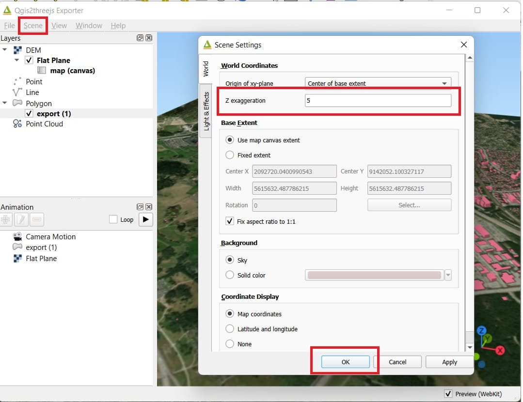
Do you see any difference? Probably not! Why? Don’t forget the Z factor value for stretching a little bit the result and make it more impressive! We select > Scene > Scene Settings > Z exaggeration: 5.

Why the Z exaggeration is 5 and not 200 like in the DEM example? Keep in mind that the DEM example was using the Digital Elevation Model for the entire Sweden and this time, the Open Street Map (OSM) data we downloaded is for a small area in Stocholm city. So, it’s a matter of scale!

And the final result will look like this…

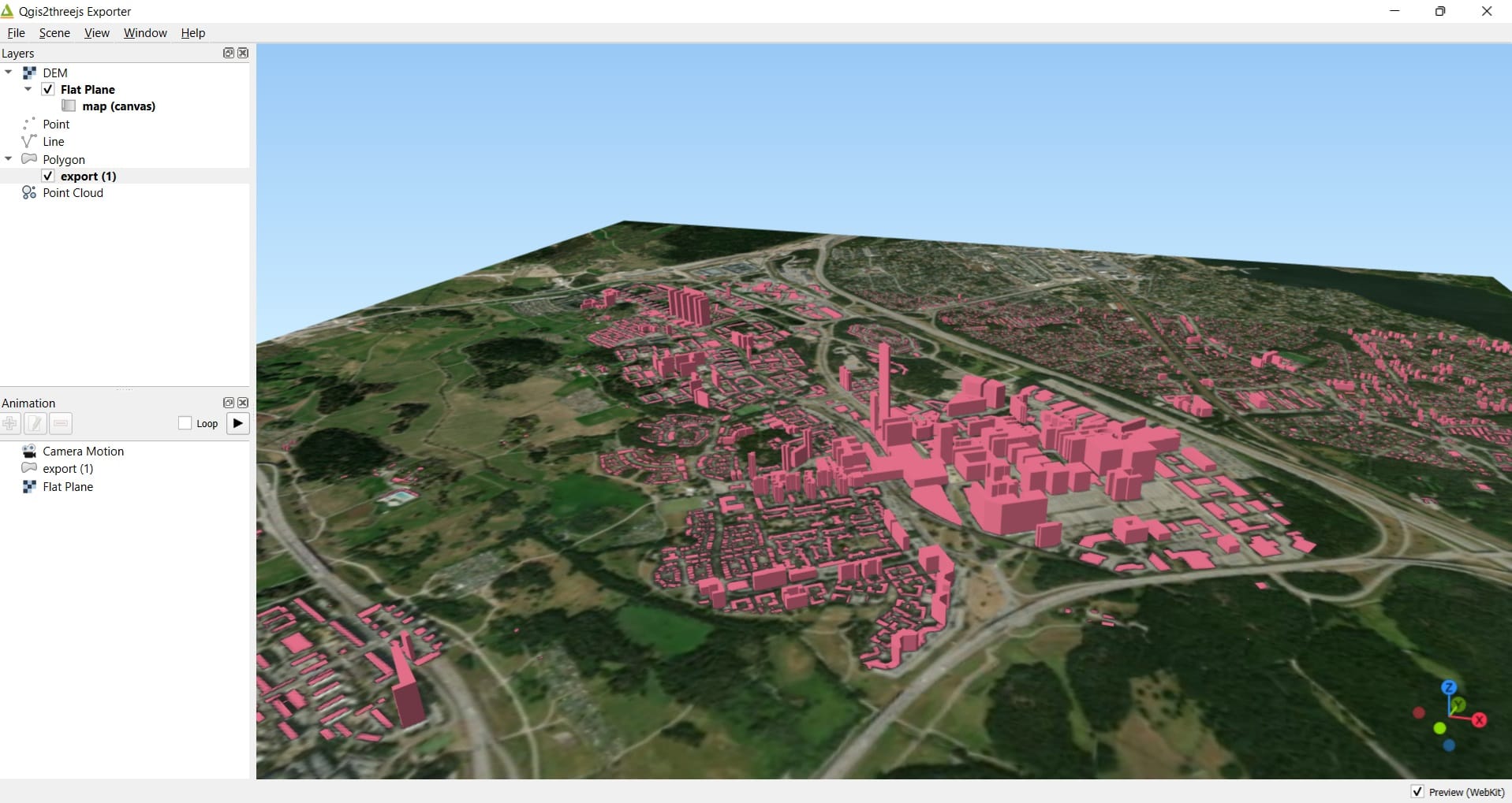
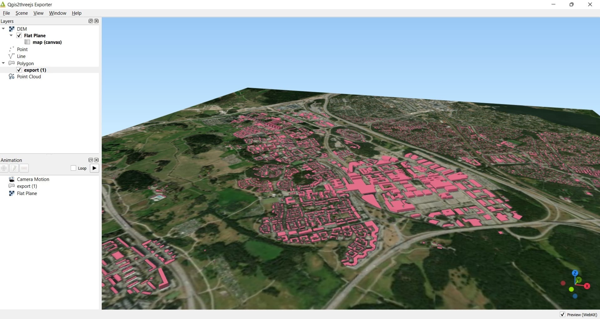
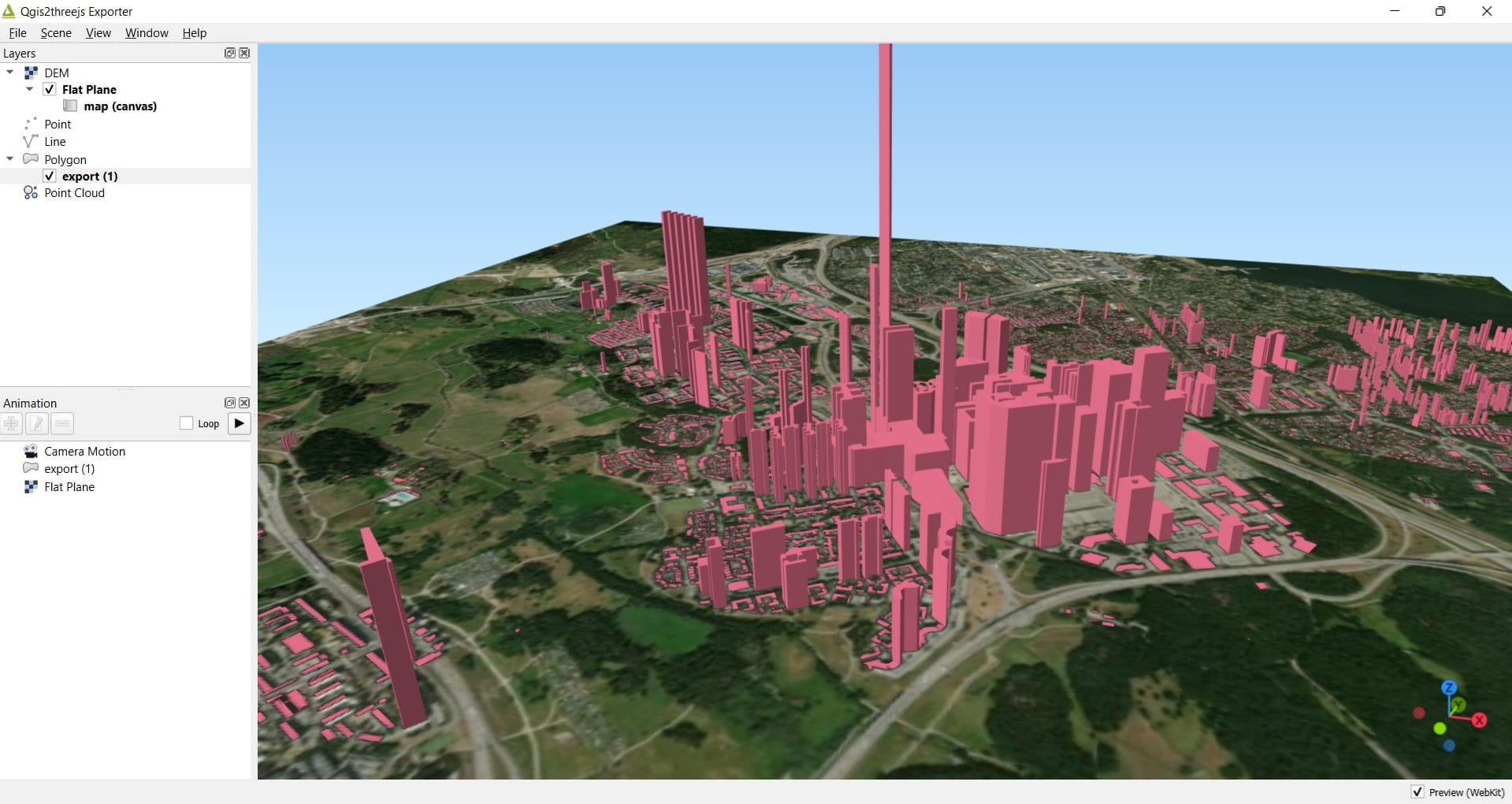
Explain to your students that the result above is a scaled result and there are no such tall buildings in these area, let them experiment with the scale factor (i.e. scale factor: 1 and 20) and identify the differences (see the images below). Scale factor: 1 is pretty much closer to the reality and a Scale factor: 20 transforms the building blocks like we live in Manhattan.

Also, you may change the buildings colors (by double-clicking in the QGIS Layers tab > export > double-click > Symbology), you may zoom-in or zoom-out and of course, you can export your 3D maps to images (.jpeg) or web files (.html) like we did in the DEM example.

For more practicing on QGIS 3D models, check the following videos! The only thing you will need is just to download some Digital Elevation Models (DEM) raster images and load the QGIS Basemaps! Good luck!