Buffer, clip and intersect vector data

Introduction to basic vector processing

In GIS, vector data processing allows us to focus our analysis on specific areas, explore spatial relationships, and extract meaningful insights from layered geographic information. In this lesson, you’ll work with three fundamental geoprocessing tools: Buffer, Clip, and Intersect.

These tools are essential for projects involving environmental planning, urban analysis, site selection, and field-based education, allowing you to define zones of influence, extract areas of interest, and identify overlapping features between datasets.

By the end of this lesson, you will:

✅ Create buffers around points, lines, or polygons to identify influence or exclusion zones (e.g. buffer around a road or a school)
✅ Use the clip tool to extract a specific geographic area from a larger dataset (e.g. your neighborhood from a national boundary layer)
✅ Apply the intersect tool to find and extract overlapping areas between different vector layers (e.g. where green areas intersect with school zones)
✅ Understand how these tools work together to support spatial decision-making and local-scale analysis
✅ Practice hands-on workflows that link spatial analysis with classroom, community, or environmental data projects

Let’s explore how to process vector data to extract what matters most from your maps! 🗺️🧩✨

🗺️ Vector processing

Vector data processing and spatial overlay is a process that allows you to identify the relationships between point, line or polygon features that share all or part of the same area. The output vector layer is a combination of the input features information. Typical spatial overlay examples are:

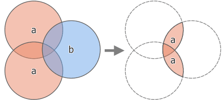
• Intersection: The output layer contains all areas where both layers overlap (intersect).
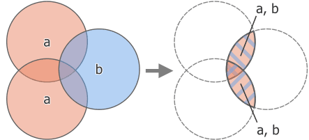
• Union: the output layer contains all areas of the two input layers combined.
• Symmetrical difference: The output layer contains all areas of the input layers except those areas where the two layers overlap (intersect).
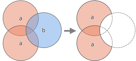
• Difference: The output layer contains all areas of the first input layer that do not overlap (intersect) with the second input layer.
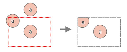
• Clip or extract by extent: Clips a vector layer using the features of an additional polygon layer. Extract by extent also creates a new vector layer that only contains features which fall within a specified extent.

In GIS Platforms, the Union, Clip, and Intersect tools are used for spatial analysis involving overlapping features. Union combines all input features into a single layer, creating new polygons where features overlap, while retaining all original attributes. Clip extracts features from an input layer that fall within the boundary of a clip layer, only keeping attributes from the input layer. Intersect creates a new layer containing only the overlapping portions of the input and clip layers, including attributes from both. You may see different examples in the images below!

 Clip                                                                                                    Difference

  Extract by mask                                                                                      Intersection

Union

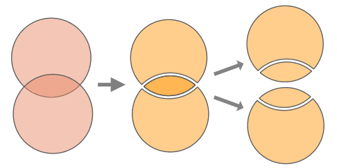
Image Source: QGIS Documentation

Another processing tool is Buffering. It usually creates two areas: one area that is within a specified distance to selected real world features and the other area that is beyond. The area that is within the specified distance is called the buffer zone. A buffer zone is any area that serves the purpose of keeping real world features distant from one another. Buffer zones are often set up to protect the environment, protect residential and commercial zones from industrial accidents or natural disasters, or to prevent violence. Common types of buffer zones may be greenbelts between residential and commercial areas, border zones between countries, noise protection zones around airports, or pollution protection zones along rivers.

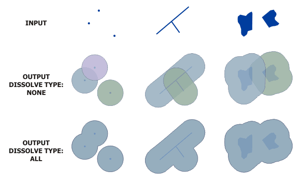
Image Source: ESRI, ArcMap Manual 

A feature can also have more than one buffer zone. A nuclear power plant may be buffered with distances of 10, 15, 25 and 30 km, thus forming multiple rings around the plant as part of an evacuation plan.

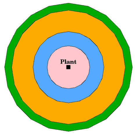
Image Source: QGIS Documentation

✨Practical exercise

Now that we explained a few concepts, let’s move to Portugal! Like in the previous lessons, the country boundaries are really important to start building our exercises.

Let’s download Portugal boundaries (i.e. polygon shapefile) via https://www.geoboundaries.org/countryDownloads.html.

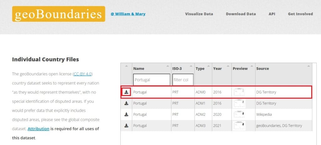
We select the ‘ADM0’ data (see the image above) and we copy and extract (unzip) the data to our ‘GIS_Training’ folder. You can create a new sub-folder named ‘Portugal’ and a new QGIS project as well.

Next, we will download some environmental data in shapefile format. Let’s try to download all Natura areas (protected areas) of Europe from the Europe Environment Agency Datahub! Use the following link:

https://www.eea.europa.eu/en/datahub/datahubitem-view/6fc8ad2d-195d-40f4-bdec-576e7d1268e4

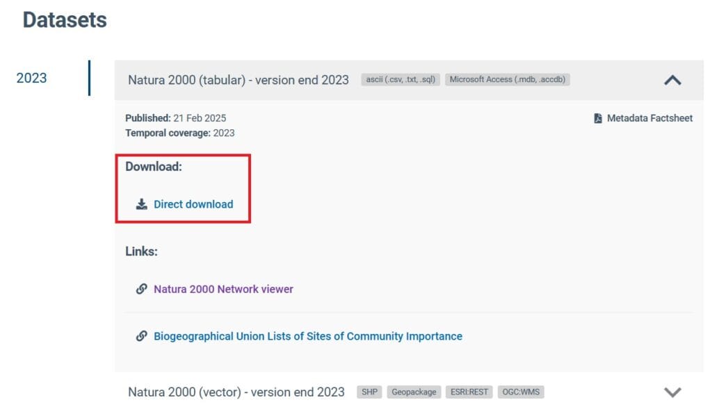
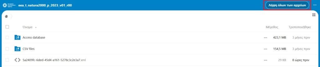
We select the ‘Direct download’ option and a new window will appear (see the image below). We press ‘Download all files’ and our Natura areas data will be downloaded (ok, it will take some time).

Similarly to the geoBoundaries shapefile data, we copy the Natura file to the ‘GIS Training’ folder > ‘Portugal’ and we extract all files.

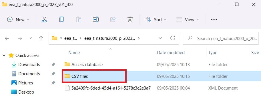
In the ‘eea_t_natura2000_p_2023’ file we have extracted, you may find different sub-folders. One of them is ‘CSV files’. Does it remind you of something?

There are no shapefiles in the data we’ve downloaded. However, if you remember from our previous lesson, we can load .csv data that include the coordinates (i.e. latitude/longitude) information. Let’s load all Natura areas of Europe as point data!

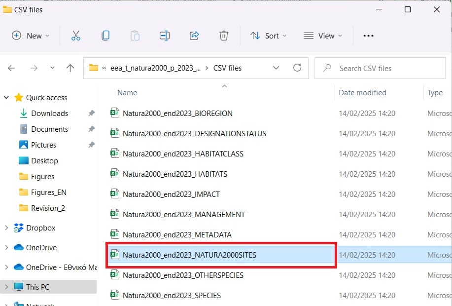
The .csv we are going to load on QGIS is the ‘Natura2000_end2023_NATURA2000SITES’ file. If you remember, on QGIS we select on the main toolbar on top ‘Layer’ > ‘Add Layer’ > ‘Add Delimited Text Layer’ and then, you select the .csv file you want to load (see the image below).

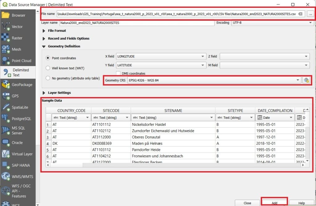
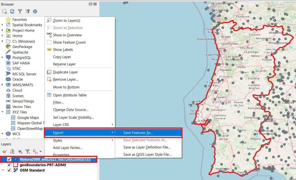
You don’t have to change or modify anything, after you load the .csv file, just press ‘Add’! After you load the .csv file, all Natura areas will be visualized (as points). Keep in mind that this is not a shapefile yet, it’s just a .csv file we’ve loaded. If you want to save these data permantly as a shapefile, just right-click on the file (Layers window) > ‘Export’ > ‘Save Feature As’ and save your shapefile in the ‘GIS_Training’ > ‘Portugal’ folder with the name ‘Natura_Europe’.

Now that we have both the Portugal boundaries and the Europe Natura areas data, we can start our processing! A first try is to clip (remove) all Naura areas for the rest of the European countries and keep the Natura areas for Portugal. In GIS, there are 2 options to do that, either by clipping one layer to the extend (the boundaries) of another one or by intersecting 2 layers (extract the features that are included inside the boundaries of one layer/shapefile).

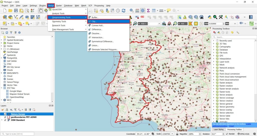
Let’s try the ‘Clip’ method! Keep in mind that we are working with shapefiles (Vector data) so, all the processing tools we need can be found on the ‘Vector’ tab of QGIS main toolbar.

Thus, we select ‘Vector’ > ‘Geoprocessing Tools’ > ‘Clip’.

All these tools have more or less the same logic, first we select the shapefile (Input Layer) we want to process, then the shapefile to clip our data (Overlay Layer) and then, the folder we want to save our new shapefiles (let’s name it ‘Natura_Portugal’, see the image below).

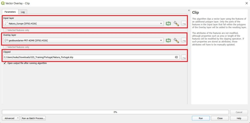
If we press ‘Run’ we’ll get the following result. You may also de-activate the ‘Natura_Europe’ and the ‘OSM_Standard’ layers.

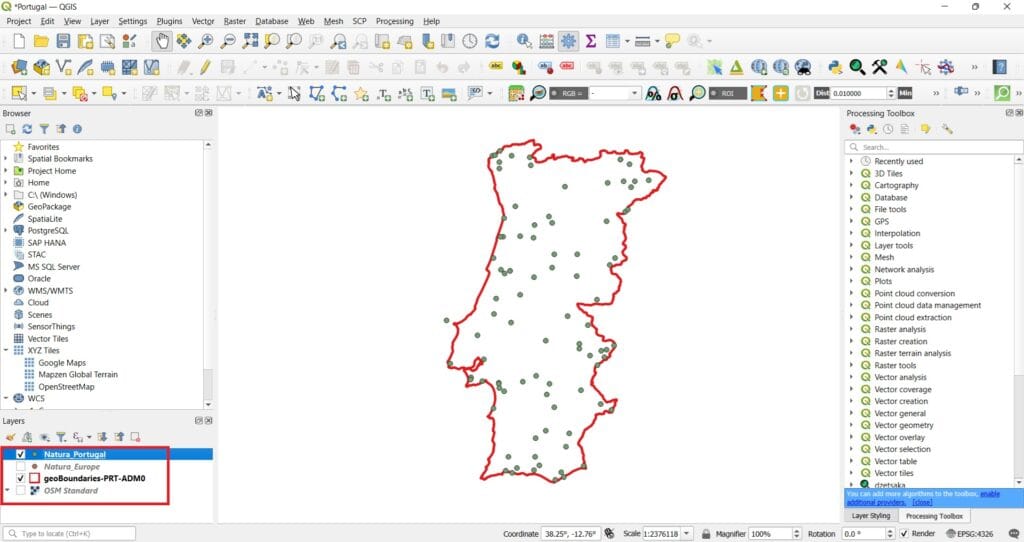
Do you see the green dot on the western coasts of Portugal that seems to fall outside the boundaries? How is that possible? Let’s zoom-in.

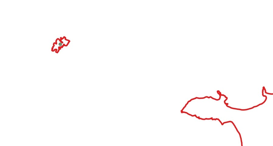
There is a tiny polygon there too! That’s why the clip function kept this point Natura area (Reserva Natural das Berlengas). Remember, we asked for those points that are inside ALL POLYGONS of our boundary shapefile!

Let’s try another processing tool! For example, the ‘Buffer’ tool. What a buffer is? A buffer zone is an area of specified distance or time around one or more features [1]. For example, to protect an endangered species, construction activity is not allowed within a 1000-meters buffer of its habitat. We can try this scenarion with the ‘Natura_Portugal’ point shapefile! Let’s try to save some endagered species within a zone (buffer) of 20000-meters (or 20 kilometers)!

Before we do that, we should consider that all data we have downloaded have the same Coordinate Reference System (CRS) which is…….WGS 84 (EPSG: 4326). This means that all measures are in degrees (not in meters!!!!). Thus, if we want to use the ‘Buffer’ tool, we have 2 options:

• Reproject our ‘Natura_Portugal’ shapefile to a projected coordinate system (i.e. ETRS89 / Portugal TM06 EPSG:3763)
• Transform the 500 meters buffer zone from meters to degrees (it’s too risky and let’s say more complicated to approximate this calculation)

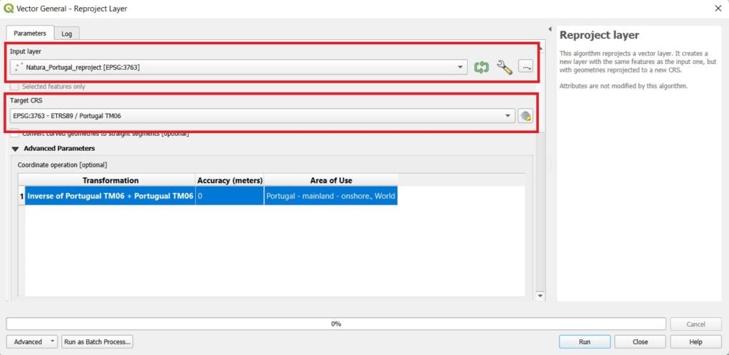
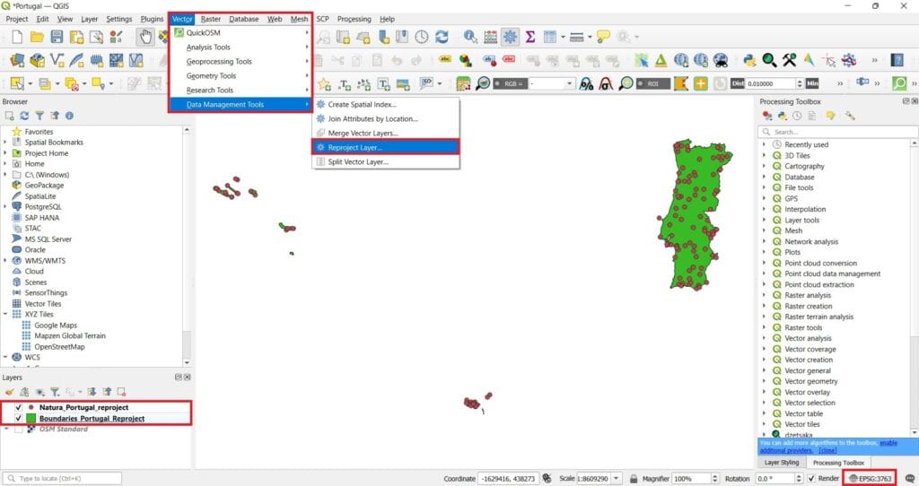
Let’s try the first option since we saw the first one in the previous lesson and you already know how to reproject a Vector dataset. You can use the ‘Reproject’ tool on the main QGIS toolbar (see the image below) and run the tool 2 times, one for the Natura areas and one for the Portugal boundaries. Name the new files (scroll down on the Reproject Layer tool to set the folder and the name) as ‘Natura_Portugal_Reproject’ and ‘Boundaries_Portugal_Reproject’.

Don’t forget to change the CRS on the bottom-right corner of QGIS (see the image below) and set the ‘ETRS89 / Portugal TM06 EPSG:3763’ as the project CRS.

If you compare the size and the shape of Portugal woth the WGS 84 CRS, you may find some differences (see the previous images above). Portugal looks larger on the Y axis and slightly thinner on the X axis. That’s normal! If you remember from the previous lessons, different projection systems show distortions of angular conformity, distance and area.

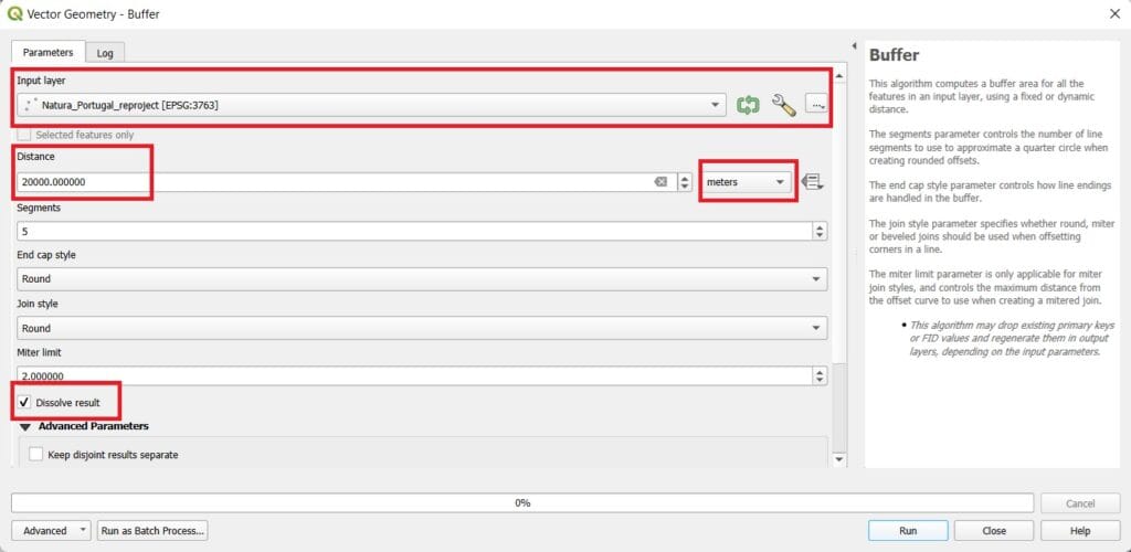
Now let’s try to protect some species by creating our buffer zones! We select ‘Vector’ > ‘Geoprocessing Tools’ > ‘Buffer’.

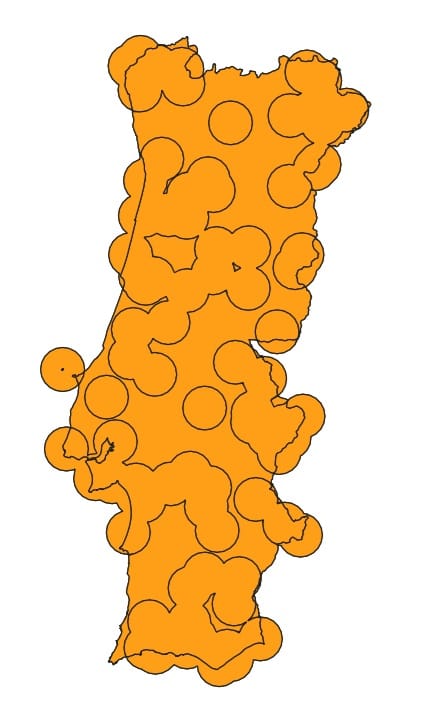
As ‘Input layer’ we select the ‘Natura_Portugal_Reproject’, we set a distance of ‘20000’ meters (you may change the distance metrics), we enable the ‘Dissolve result’ checkbox and finally, we save our file as ‘Safe_Areas’!

But, what the ‘Dissolve result’ checkbox does? Dissolve tool/selection aggregates features based on specified attributes. Dissolving is mainly for generalization and always simplifies boundaries from a more complex one [2].

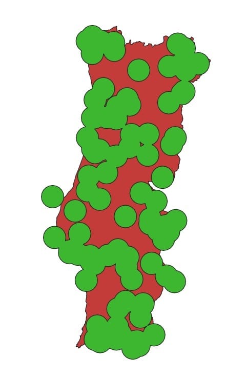
Our result will look like this. Our safe areas are illustrated as green polygons (combinations of circles). You may change the colour by double-clicking on the resulted file (‘Safe_Areas’) and changing the ‘Symbology’ colours.

If you don’t check the ‘Dissolve result’ checkbox, the resulted buffer zones will not be dissolved and the result will be slightly different like in the image below.

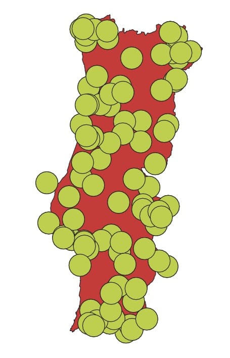
The buffer zones are the same however, they are not ‘merged’/dissolved and they can be seen as different areas. Keep in mind that an alternative option instead of using the ‘Clip’ tool is the ‘Intersection’ tool. Same logic and the same result!

And what if we want to merge 2 polygon feature classes (datasets) or 2 point or 2 line feature classes? Of course we can do it! Let’s try the ‘Union’ tool for merging the Portugal boundaries and the Safe areas!

This time, we will use the ‘Vector’ > ‘Geoprocessing Tools’ > ‘Union’.

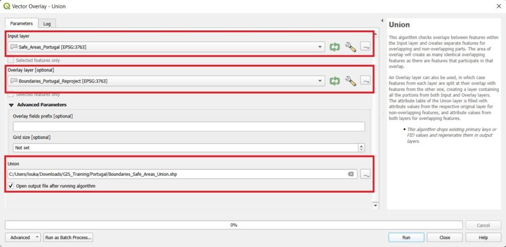
‘Input Layer’ is our ‘Safe_Areas_Portugal’ layer, ‘Overlay Layer’ is the ‘Boundaries_Portugal_Reproject’ layer and we save the merged layer as ‘Boundaries_Safe_Areas_Union’. The result will look like in the image below.

✅ Wrapping Up

You’ve just completed the lesson on how to Buffer, Clip, and Intersect vector data in QGIS—three essential tools in any GIS workflow. These operations help you focus your analysis, define zones of influence, and extract meaningful spatial relationships between datasets.

Whether you’re working on a school project, an urban planning task, or an environmental study, mastering these tools empowers you to make informed, location-based decisions. You may also take a look on the following videos explaining different vector processing capabilities!

In the next lesson, we’ll continue building your spatial analysis skills with even more powerful raster tools.
Great work! Keep exploring and processing! 🌍📐🗺️