Basic raster processing capabilities

🌄 Introduction to Basic Raster Processing in QGIS

Raster data—such as satellite imagery, digital elevation models (DEMs), or land cover maps—is a powerful source of spatial information. Unlike vector data, raster files are made up of grids of cells (pixels), each with a specific value that represents information such as elevation, temperature, vegetation index, or land use.

In this lesson, you’ll explore basic raster processing tools that allow you to prepare, analyze, and visualize raster data for your GIS projects. These skills are fundamental when working with environmental data, remote sensing imagery, or terrain models.

By the end of this lesson, you will:

✅ Learn how to clip raster layers to focus on your area of interest (e.g. city, region, or school zone)
✅ Understand how to reclassify raster data by changing or grouping cell values for better interpretation
✅ Use raster calculator and map algebra to perform basic mathematical operations on raster layers
✅ Understand how to rasterize vector layers and convert raster data into visual, meaningful formats

With these tools, you’ll be able to transform raw raster files into actionable maps that support classroom activities, environmental analysis, and spatial storytelling.

Let’s begin exploring the grid-based world of raster data! 🛰️📊🗺️

This time we travel to France and we will try to download first some raster data both for the inshore and the offshore areas of France.

Step 1: Download wind and elevation data from Global Wind Atlas (link).

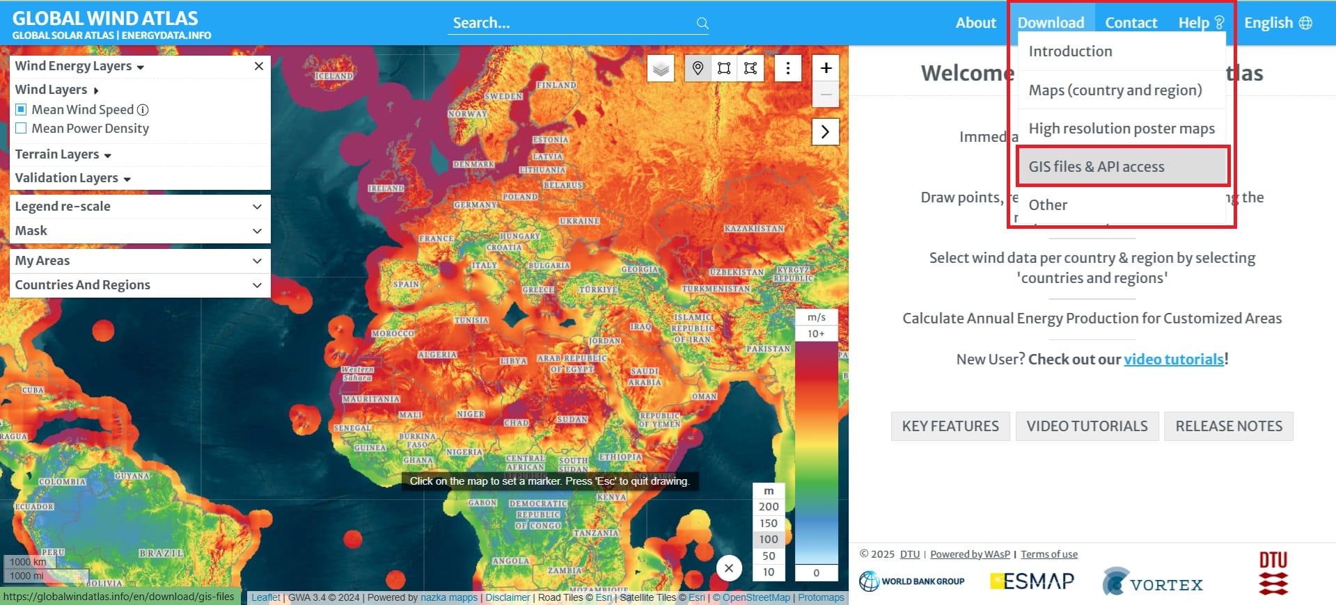
We select ‘Download’ > ‘GIS files & API access’, then choose ‘France’ in the Country field, ‘WIND-SPEED’ in the Select Layer field, and either ‘100’ or “150” in the Select Height field (it depends on how high we want our wind turbines to be but, we will work on that in the upcoming lessons).

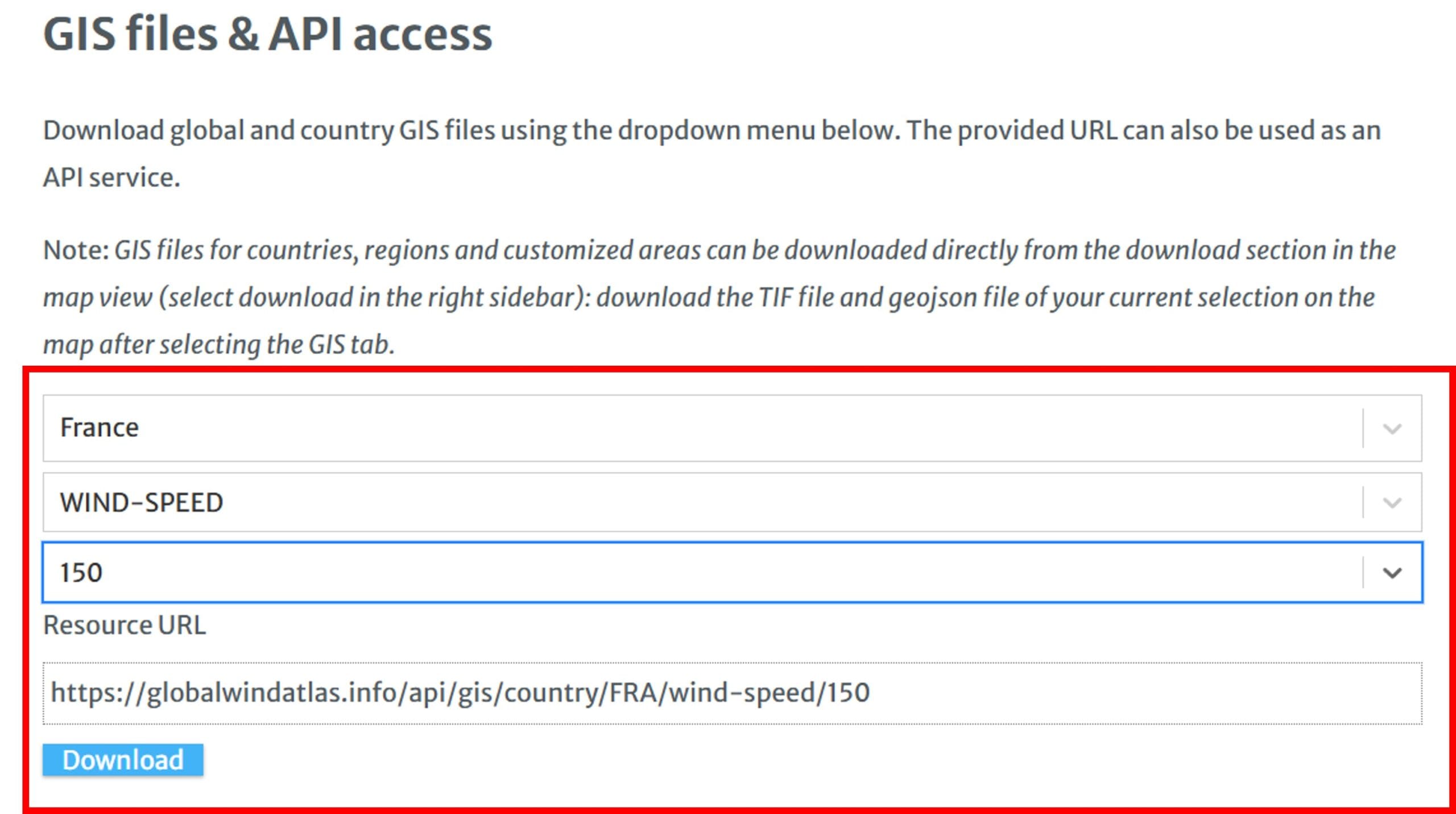
We follow the same process to download the bathymetry-elevation data.

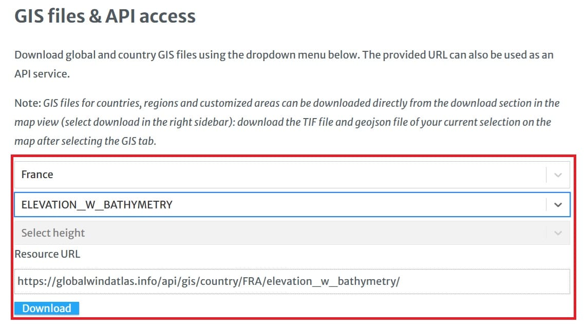
Step 2: We will download some shapefile data (boundaries) of France in order to be able to process our raster data.

Let’s try first the Exclusive Economic Zone (EEZ) boundaries of France via the Marine Regions website (link)! When you open the link, you scroll down and you select to download the EEZ boundaries in shapefile format!

Step 3: Let’s download the Natura areas of France but this time, in polygons (shapefile format)!

You may use the national spatial data portal of France via this link.

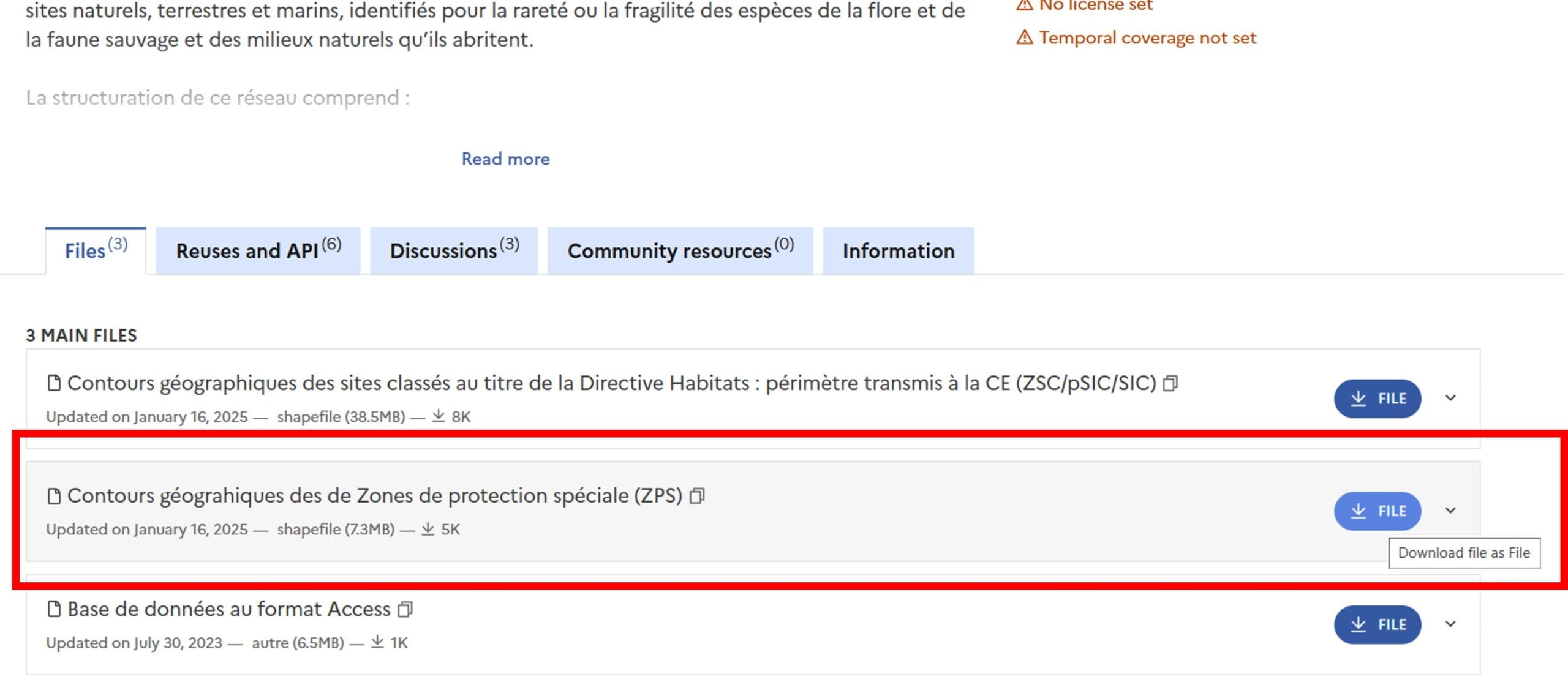
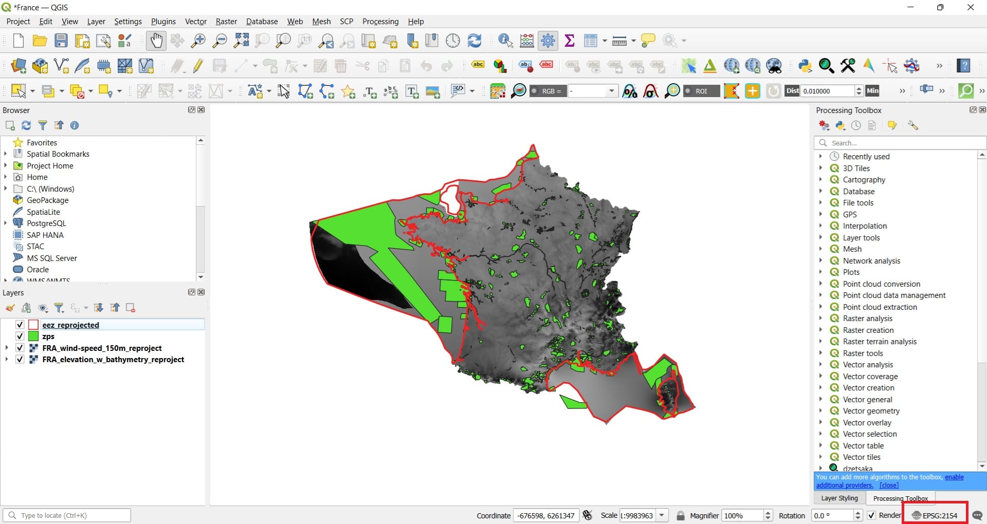
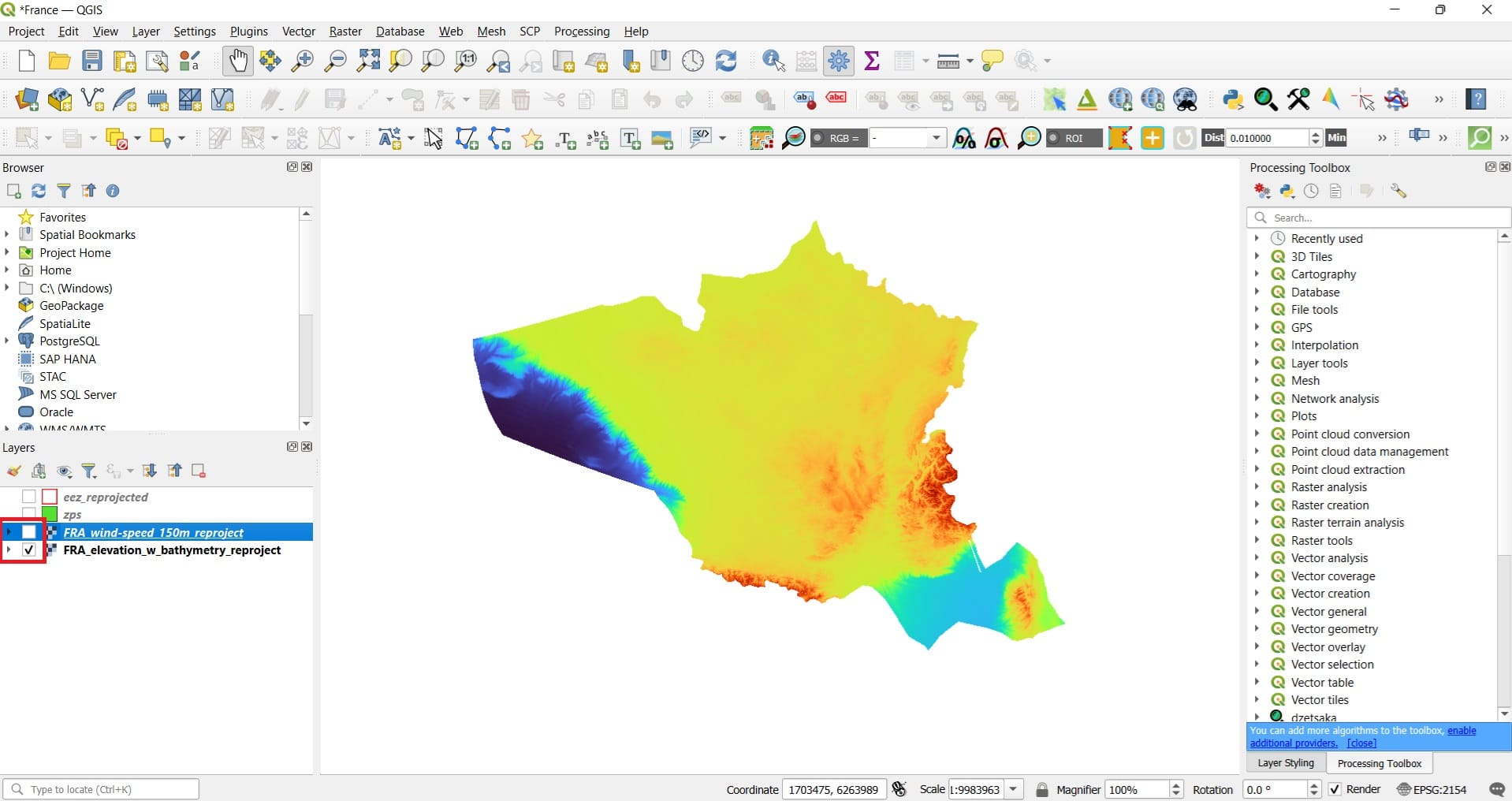
You may copy all data we have downloaded to a new folder (i.e. folder France) in ‘GIS_Training’, unzip both the ‘eez’ and the ‘zps’ (Natura France) files and open a new QGIS project by saving it as ‘France’. The wind and the elevation-bathymetry files are not compressed so, you can just copy them in .tiff format to the new folder! Let’s load all data on QGIS.

Important note:

• In order to load your vector data (i.e. ‘zps’, ‘eez’), you select ‘Layer’ > ‘Add Layer’ > ‘Add Vector Layer’
• In order to load your raster data (i.e. ‘FRA_elevation_w_bathymetry’,’FRA_wind_speed_150m), you select ‘Layer’ > ‘Add Layer’ > ‘Add Raster Layer’

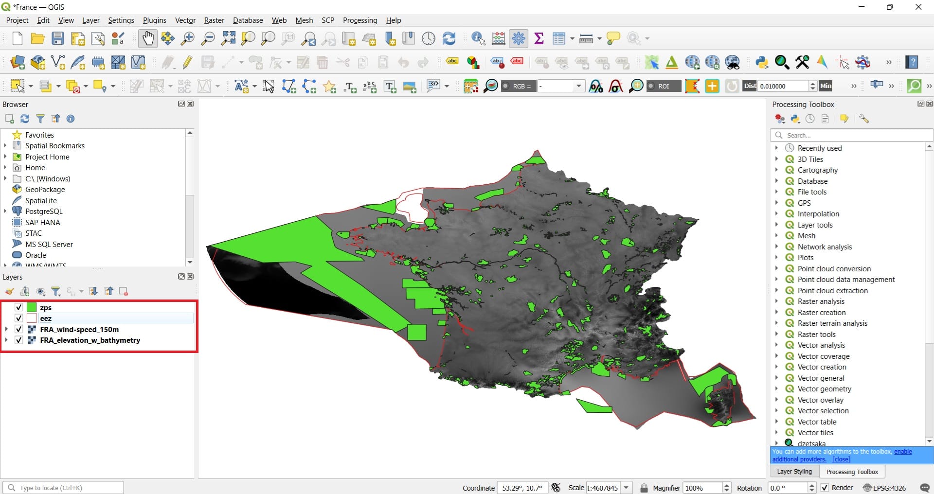
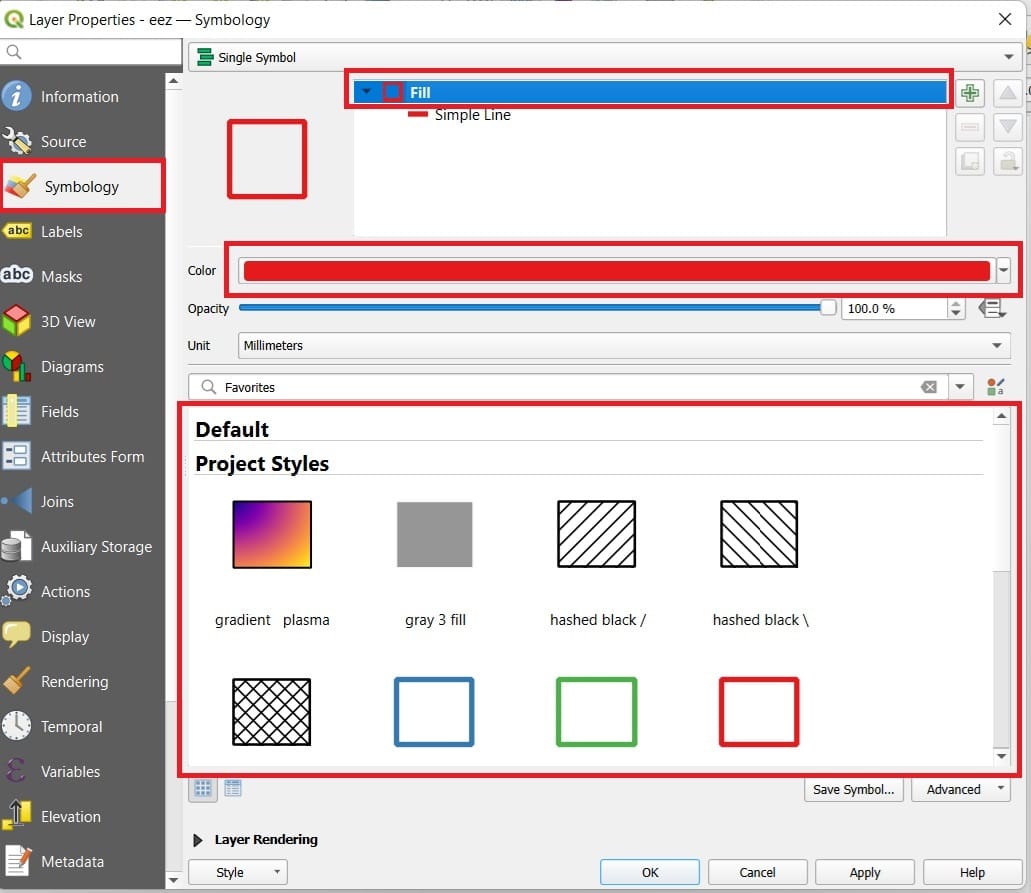
You may also change the Symbology (colours) of the ‘eez’ vector layer by double-clicking on it > ‘Symbology’ > Option 1: Default style or Option 2: Click on the ‘Color’ and reduce the opacity to 0%.

Before we start do you remember what is the first check we should do?

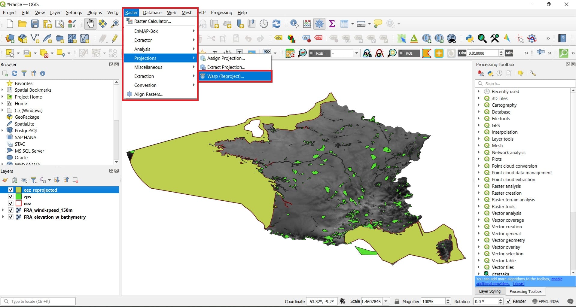
That’s right, we must the the Coordinate Reference Systems (CRS) of our data! By double-clicking on each one of our shapefile and tiff files > ‘Source’ we will find out that the ‘zps’ shapefile uses the ‘EPSG:2154 – RGF93 v1 / Lambert-93’ and all the remaining data are using the ‘EPSG:4326 – WGS 84’. Why? Because if you remember, the Natura areas shapefile was downloaded by a French geospatial data portal.

EPSG:2154 is a Projected Coordinate System and EPSG:4326 is a Geographic one. Let’s project all of our data to the EPSG:2154!

For our shapefile data (i.e. the ‘eez’) we select ‘Vector’ on the main QGIS toolbar > ‘Data Management Tools’ > ‘Reproject Layer’, like we did in the previous lesson.

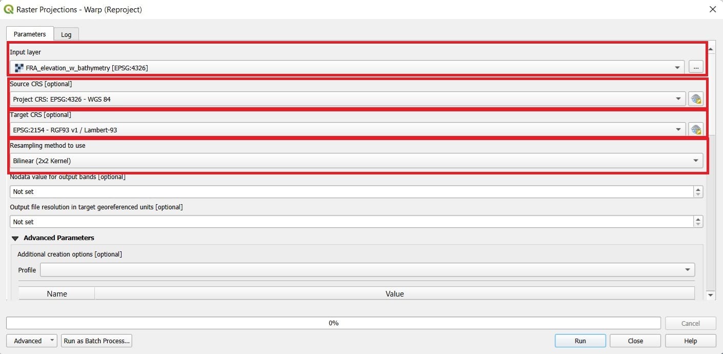
For our raster data we select ‘Raster’ on the main QGIS toolbar > ‘Projections’ > ‘Warp (Reproject)’.

In the ‘Warp (Reproject)’ tool we select:

• Input layer: ‘FRA_elevation_w_bathymetry’
• Source CRS: ‘EPSG: 4326’ (we know that because we’ve checked the Source of our data)
• Target CRS: ‘EPSG: 2154’ (the same projected CRS as the ‘zps’ data)
• Resampling method to use: Bilinear
• Scroll down and save your new file (Save as File) with the name ‘FRA_elevation_w_bathymetry_reproject’
• Press ‘Run’
• Follow the same procesure for the wind file and save as ‘FRA_wind-speed_150_reproject’

Don’t forget to set the project CRS as EPSG: 2154 in the bottom right corner of QGIS (see the image below)! Now we see how the size of France has changed compared to the WGS 84 CRS. Let’s start our processing!

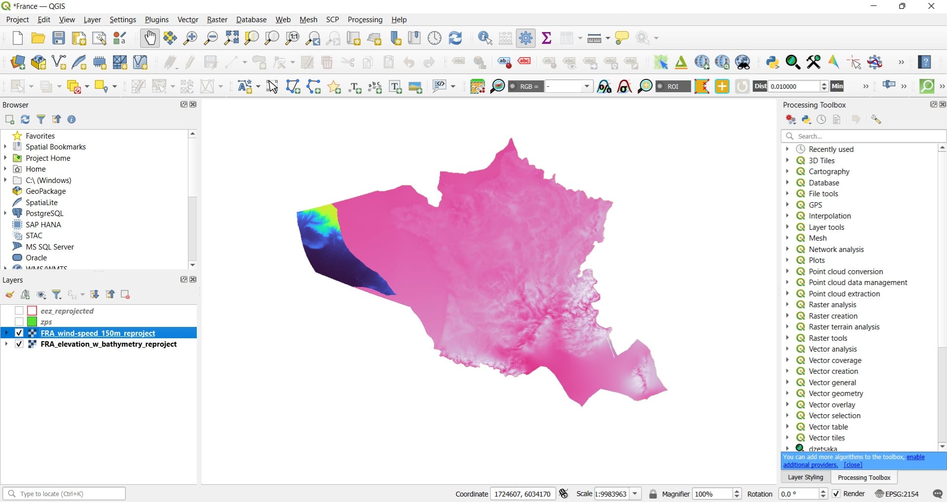
First, we can change the symbology of our rasters to enhance the visual appeal of our data! We double-click on the wind raster first > ‘Symbology’ > we select ‘Singleband Pseudocolor’ on top > we select the ‘Color ramp’ arrow and we choose > ‘PuRd’ for our wind data (dark pink for strong winds, light pink to white for lower wind speeds).

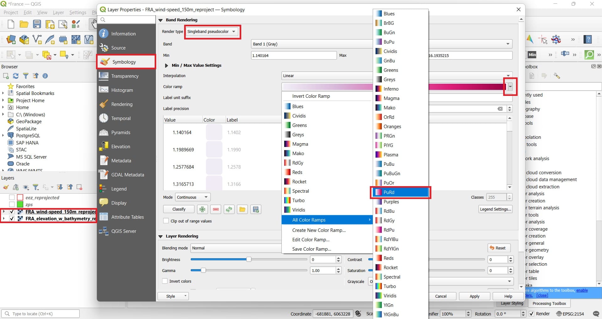
We follow the same process for the elevation-bathymetry raster and we select the ‘Turbo’ color ramp! The result will look like this!

First processing idea! Let’s suppose that we only need spatial information for the coastal and offshore areas of France! We should clip and discard the onshore areas! How to do that? We will clip both raster images using the EEZ boundaries (eez shapefile)!

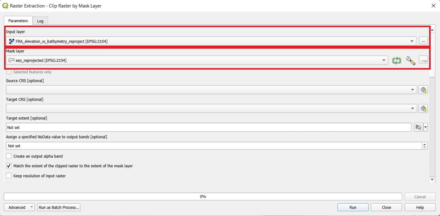
To do that, we select ‘Raster’ > ‘Extraction’ > ‘Clip Raster by Mask Layer’.

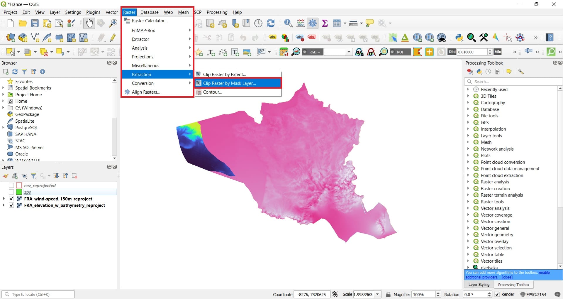
In the ‘Clip Raster by Mask Layer’ we select:

• Input layer: FRA_elevation_w_bathymetry_reproject
• Mask layer: eez_reprojected
• Scroll down and Save your file as: FRA_elevation_w_bathymetry_reproject_clip
• Press ‘Run’
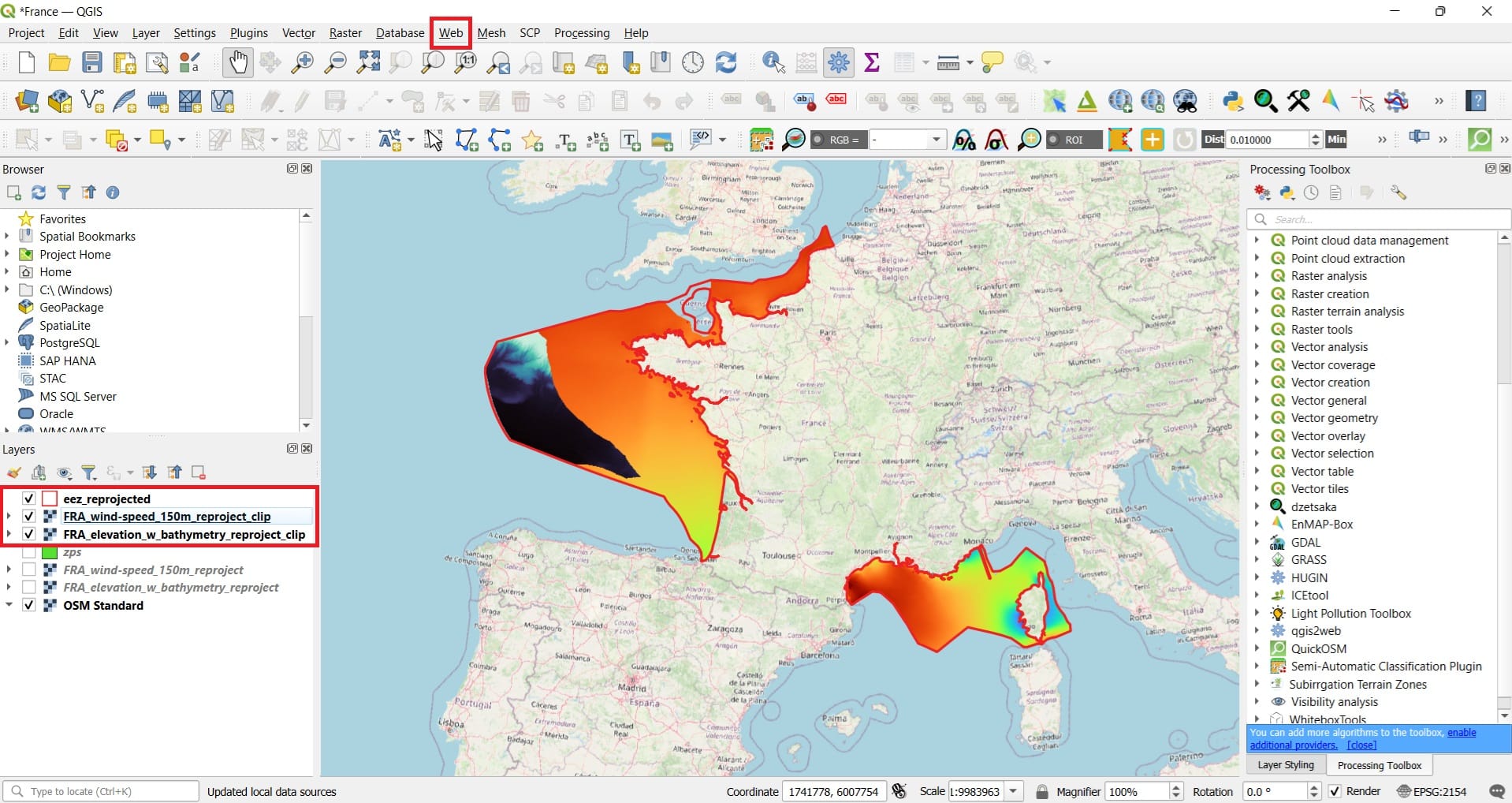
• Repeat the process for the wind/bathymetry raster and save as ‘FRA_wind-speed_150m_reproject_clip’

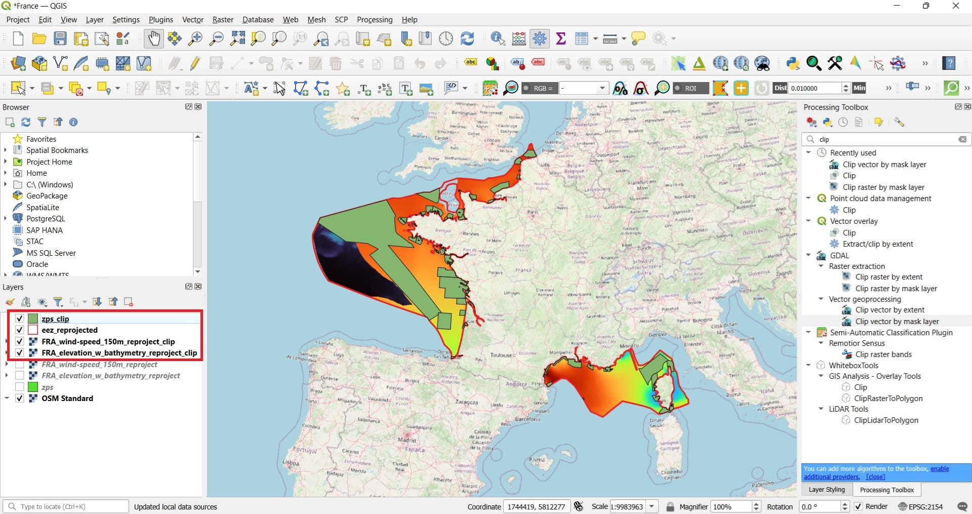
The result will look like this! We managed to discard all inshore areas of France! You may change the Symbology (colors) again and load the Open Street Map (OSM) basemap (see the image below) from the ‘Web’ tools on the main QGIS toolbar > ‘QuickMapServices’ > ‘OSM’

We can now clip our Natura areas based on the EEZ mask/boundaries. This time, we will use another ‘Clip’ tool of QGIS. Let’s type on the Processing Toolbox search bar the word ‘Clip’ (see the image below) > ‘Clip vector by mask layer’ under the GDAL tools.

But, why not to use the ‘Clip’ tool we tried on the previous lesson (‘Vector’ > ‘Geoprocessing Tools’ > ‘Clip’)? That’s a good question! Well, sometimes, we should know that in GIS platforms there are more than one ways/tools to use or follow to perform an analysis! Also, as it seems, the Natura shapefile of France has some issues, for example, some polygons have not been properly digitized and if we try to use the first Clip option, an error will occur.

Luckily, since QGIS platform is open-source, more tools have been developed from GIS experts all over the world in order to improve some tools and avoid all annoying errors for experienced and non-experienced users!

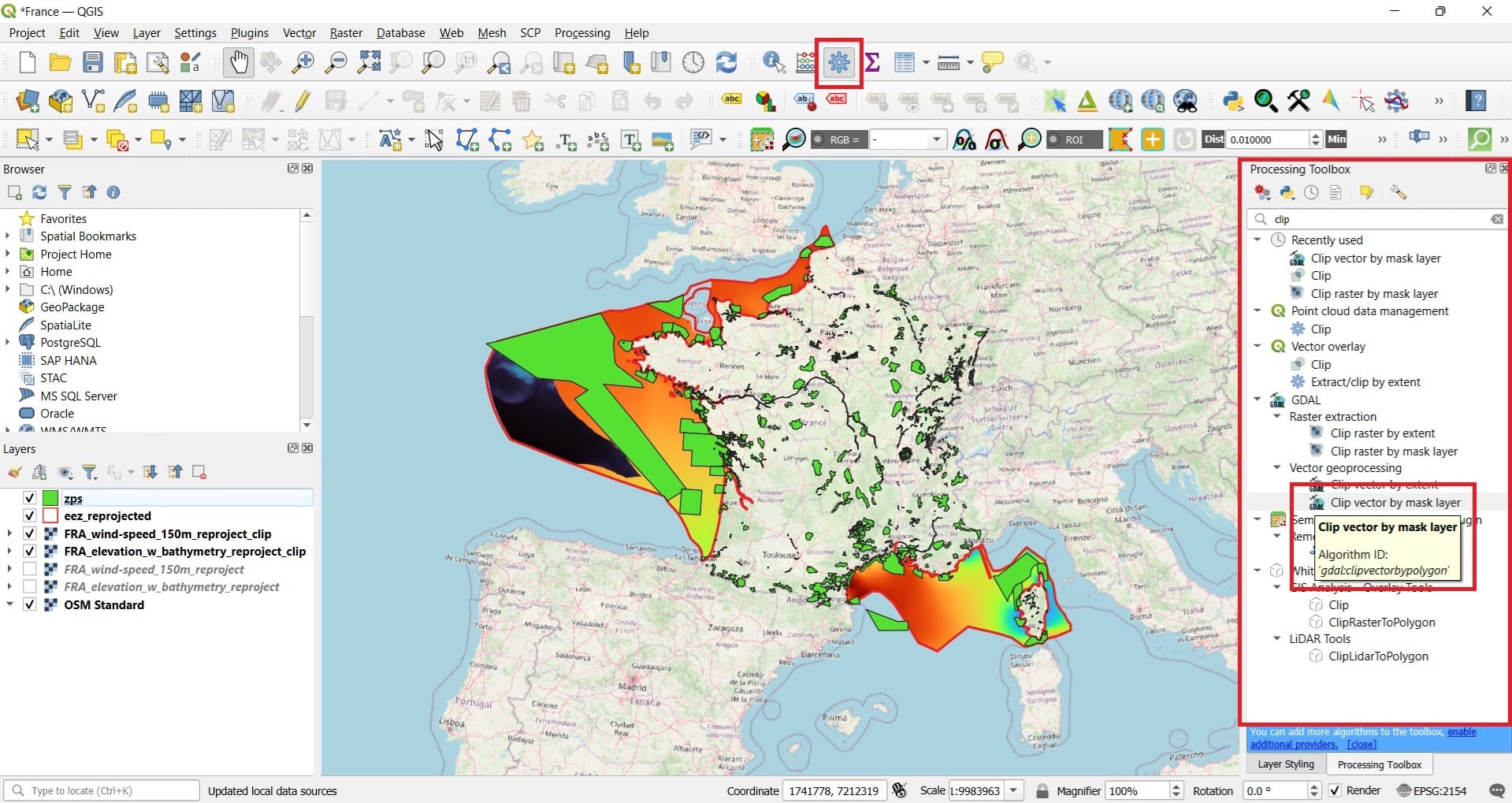
In the ‘Clip vector by mask layer’ we select:

• Input layer: zps
• Mask layer: eez_reprojected
• Clipped (mask) which is our new layer: We name it as ‘zps_clip’
• Press ‘Run’

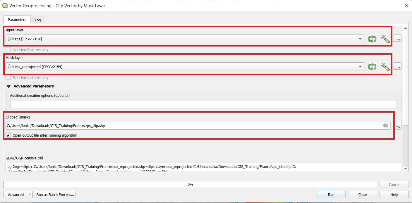
Let’s see the result! Only the offshore Natura areas have been kept and the onshore ones, have been discarded!

However, the Natura polygons is not a raster file (it’s a polygon shapefile) and in this lesson we work with raster files. This is not a problem, let’s convert it to raster! Why? We’ll find out in the next lessons!

To make the conversion, we need to collect all information needed for transforming a vector to raster, using the boundaries either of the wind or the bathymetry rasters. This information includes the number of pixels and in particular, the number of rows (height) and columns (width) that our raster image will have. If you remember from the previous lessons and courses, raster files are images with a set of pixels in rectangular form. Some pixels have no value (NoData pixels) and some others have a value assigned, for example, the wind speed, the bathymetry or any other value we can imagine.

Let’s double-click on the wind speed file and see the metadata in the ‘Information’ tab!

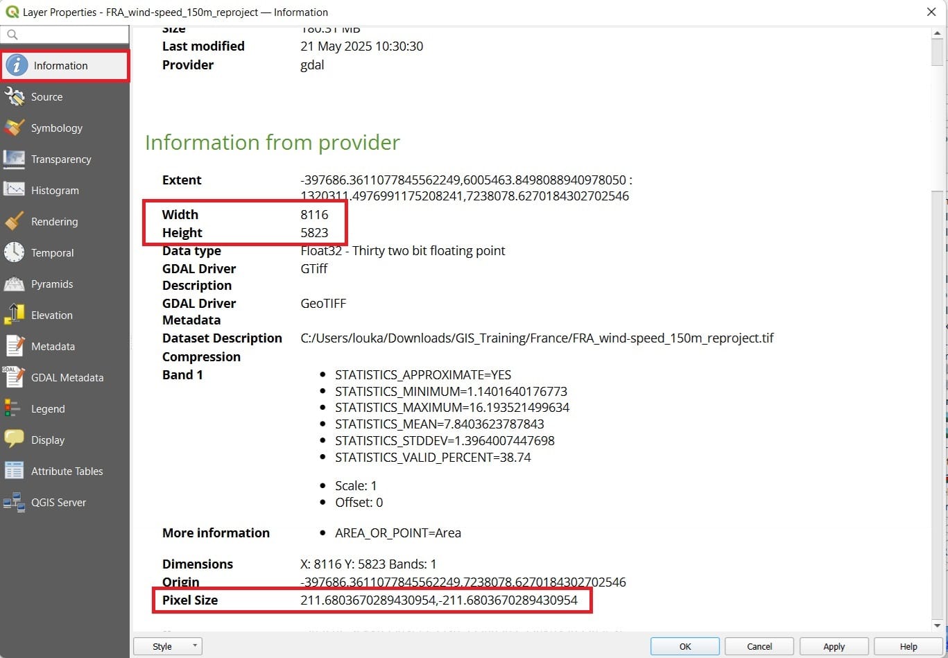
We should write down on a paper the ‘Width’ and ‘Height’ numbers:

• Width: 8116
• Height: 5823

We can now use the conversion tool we need by selecting ‘Raster’ on the main QGIS toolbar > ‘Conversion’ > ‘Rasterize (Vector to Raster)’.

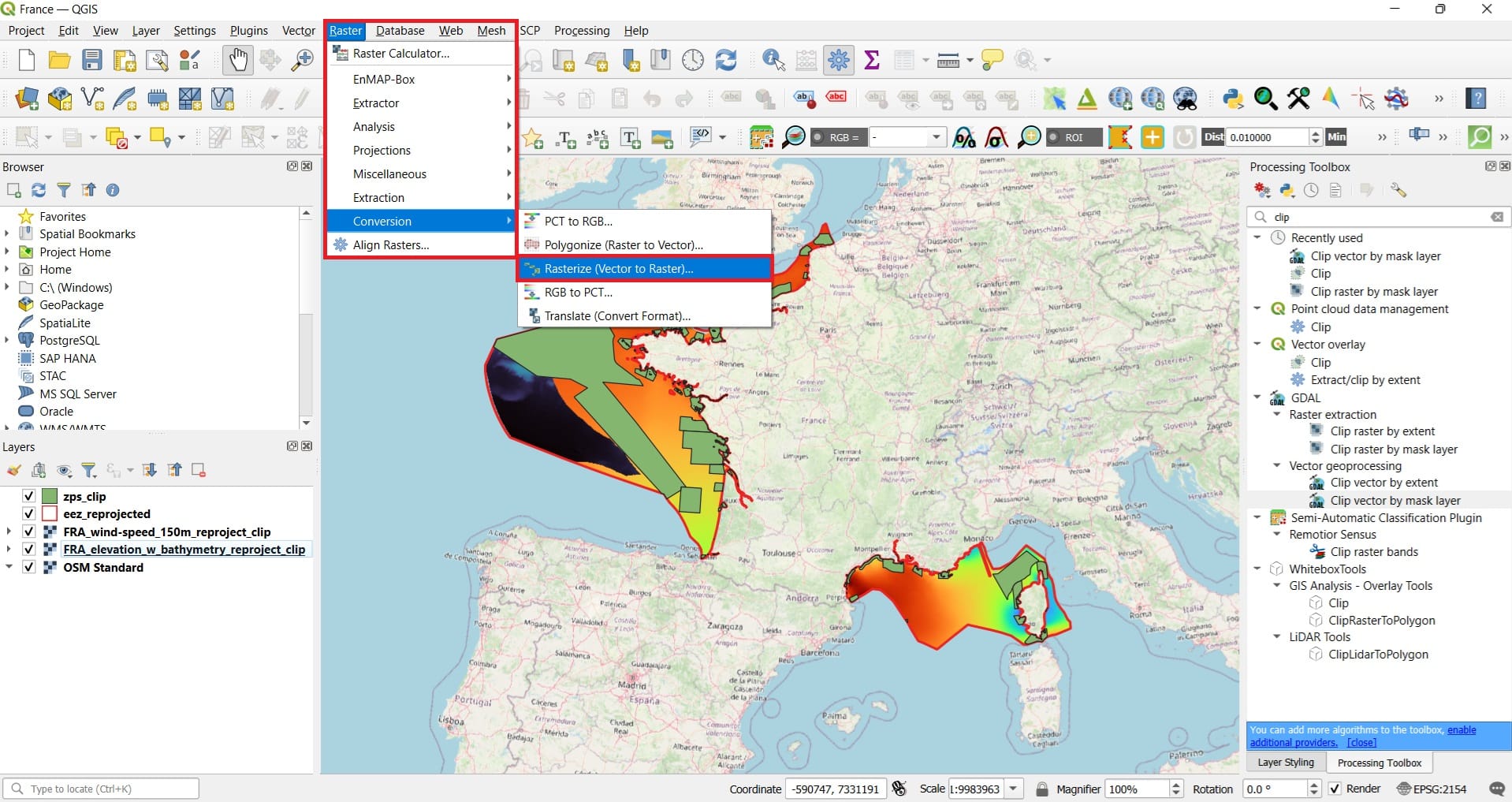
In the ‘Rasterize (Vector to Raster)’ we select:

• Input layer: zps_clip
• A fixed value to burn (metaphorically speaking): 1 (why 1? we will explain later in our lesson. It’s just a score value)
• Output raster size units: Pixels
• Width: 8116 (that’s why we needed the ‘Information’ from the wind raster)
• Height: 5823
• Output extent: ‘Calculate from Layer’ (arrow on the right) and same as the ‘FRA_wind-speed_150_reproject_clip’ (we want our Natura raster to have the same extent as the other raster layers)
• Press ‘Run’

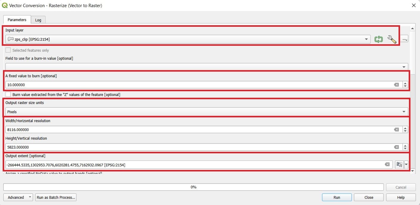
The result will look like this. The Natura areas seem to have a black color (the pixels) and a value of 1. Ok, not so impressive but, that’s an important step if we want to process all our raster files at the same time! How? Wait until the end of the course.

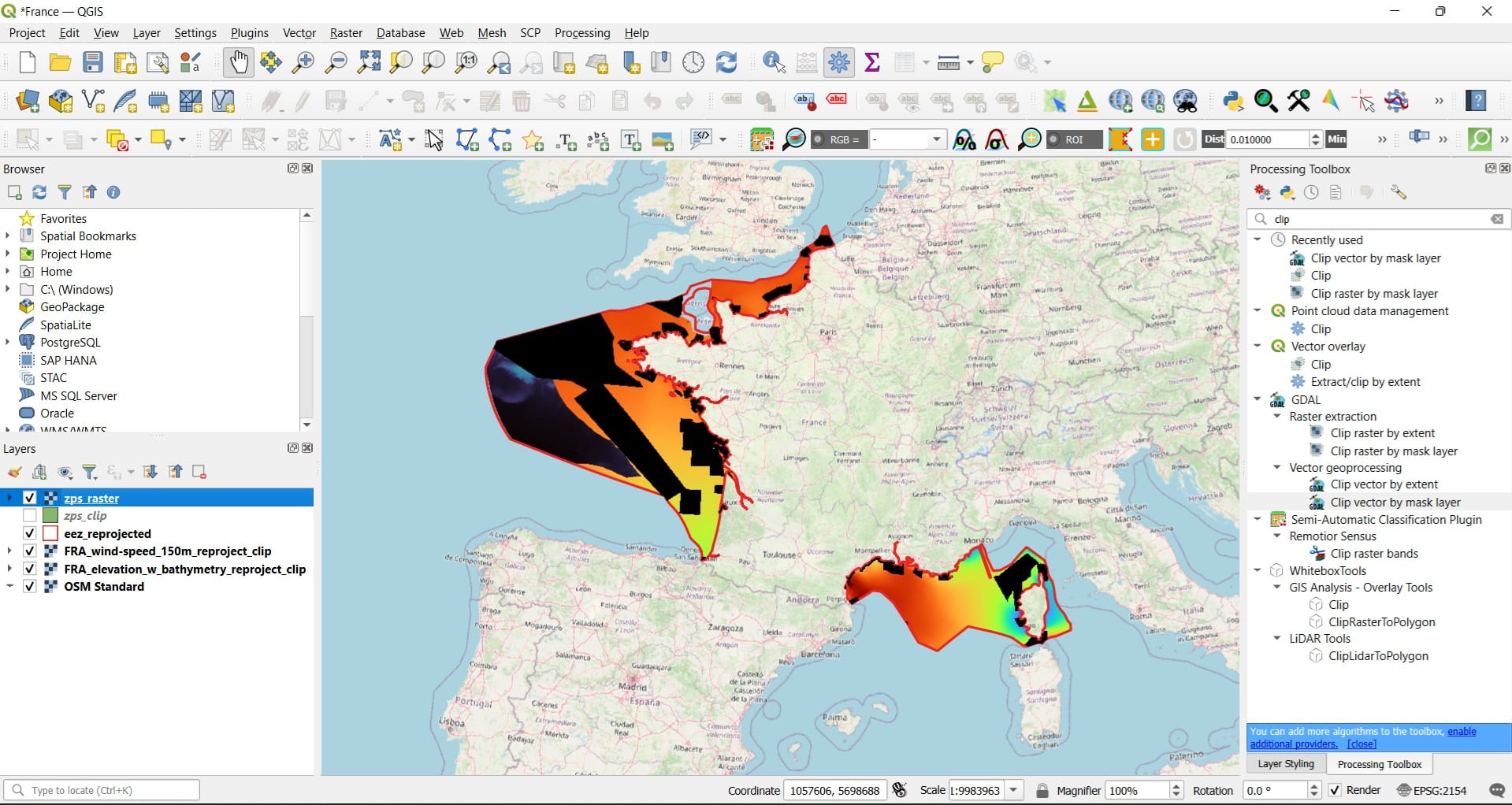
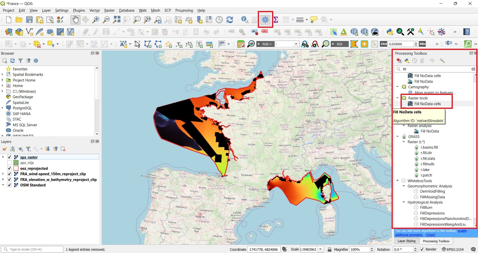
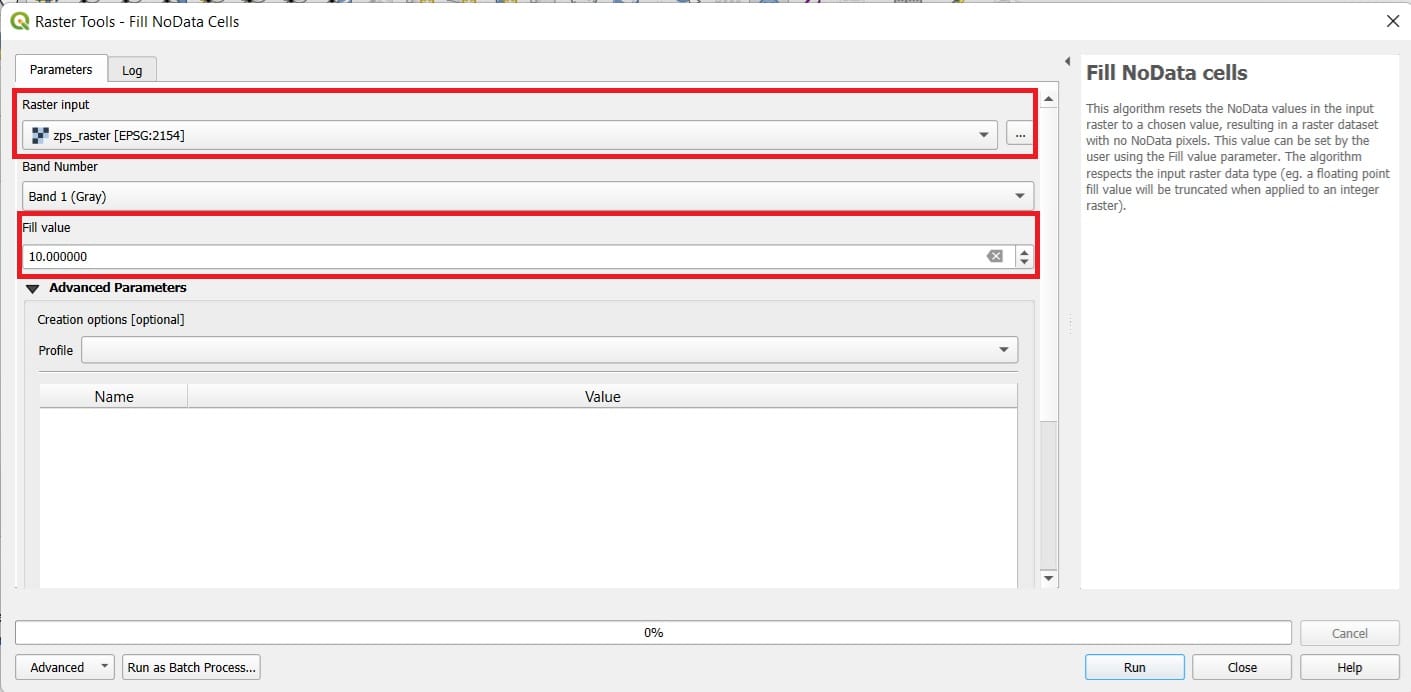
Yet, our Natura raster doesn’t look like the wind and the bathymetry rasters. It has the NoData values (the empty areas). Let’s fill these areas! Type in the ‘Processing Toolbox’ the word ‘Fill’ (see the image below) > we select the ‘Fill NoData cells’ tool under ‘Raster tools’.

In the ‘Fill NoData cells’ we select:

• Raster input: zps_raster
• Fill value: 10 (it’s just a score, inside the Natura areas we assigned 1 as a bad score and outside we assigned a value of 10 as a good score)
• Save your new file by scrolling down as ‘zps_raster_fill’
• Press ‘Run’

The result is a bit more impressive and now we realize how a raster image looks like including the NoData values. All raster images (i.e. satellite images, our TV or mobile screen look like this).

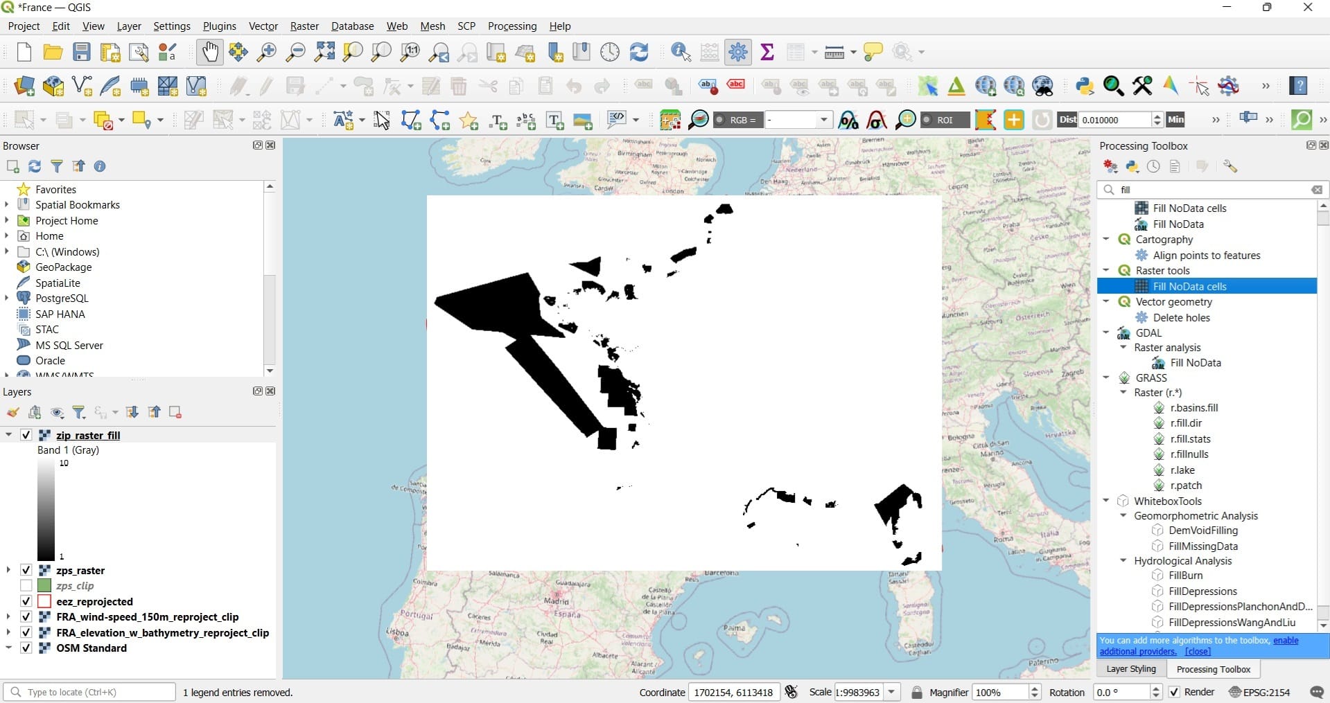
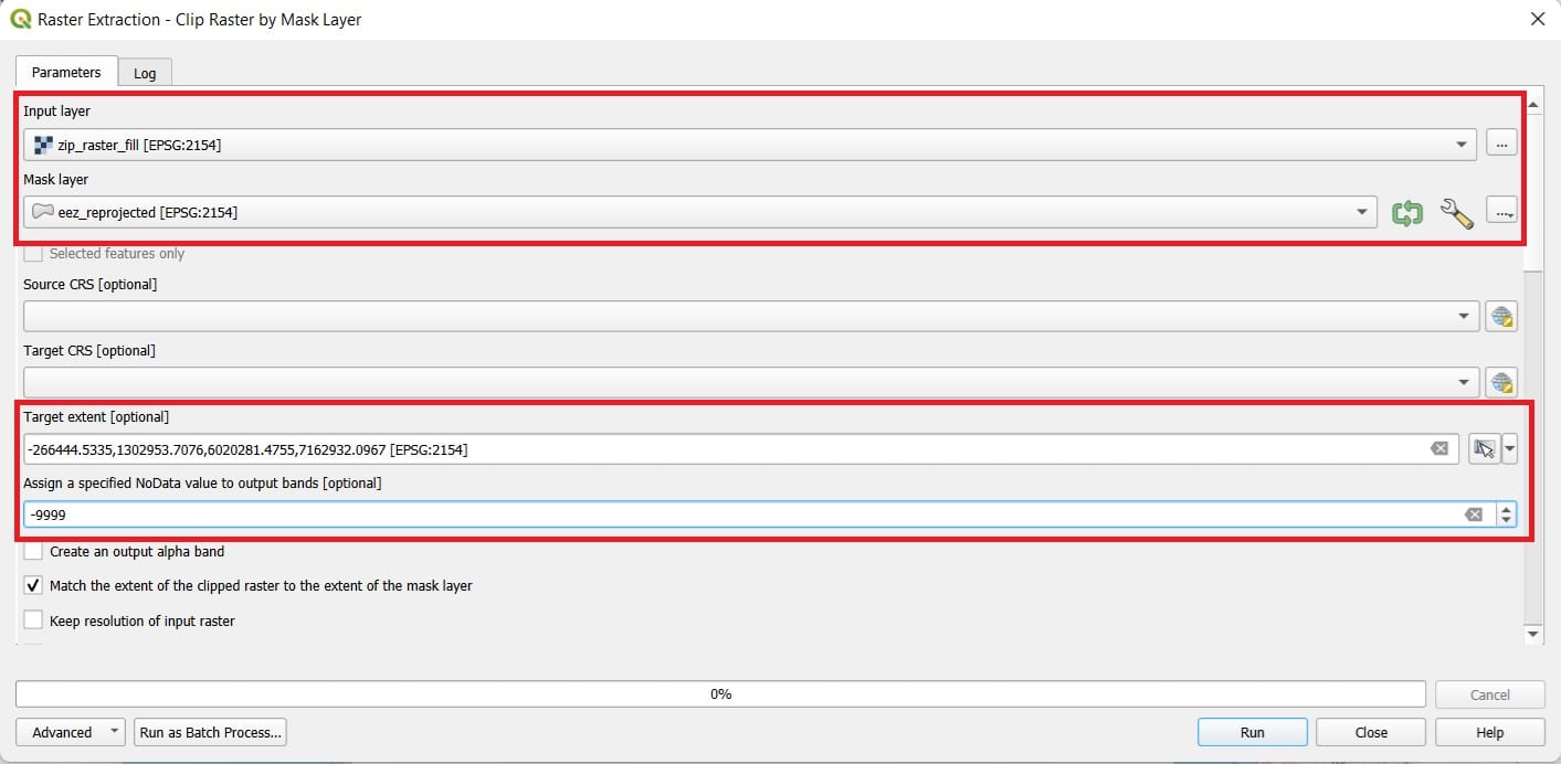
One last step? Of course! Let’s clip this image using the eez polygons like we previously did using ‘Raster’ > ‘Extraction’ > ‘Extract Layer by Mask’.

We select:

• Input layer: zip_raster_fill
• Mask layer: eez_reprojected
• Target extent: Calculate from layer (arrow on the right) and same as and same as the ‘FRA_wind-speed_150_reproject_clip’
• Assign a specified NoData value to output bands: -9999 (we want our new NoData pixels being the same as the wind raster)
• Save your file by scrolling down as ‘zps_raster_fill_clip’
• Press ‘Run’

And the result will look a bit more impressive!

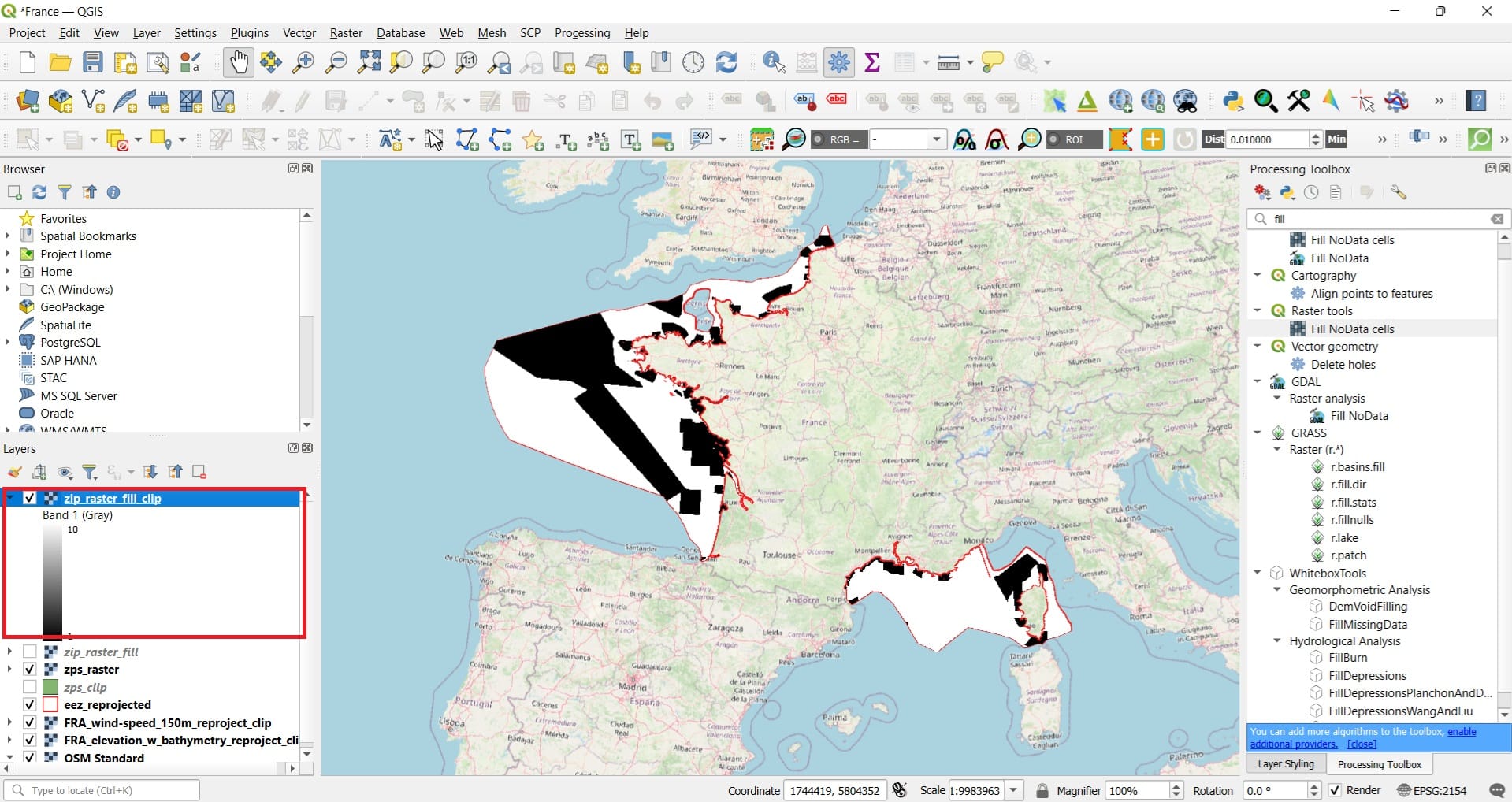
In this way, we transformed our Natura polygons to raster by assigning specific values inside and outside the polygons. Inside we have a score of 1 (bad) and outside a score of 10 (good). Why is that helping as? Just be a bit patient.

Let’s do the same for our wind and bathymetry rasters by simply using one tool and not 3 like we did with the Natura areas. We are trying to ‘translate’ the wind and bathymetry values (i.e. meters/second for wind and meters for the bathymetry) to good or bad areas.

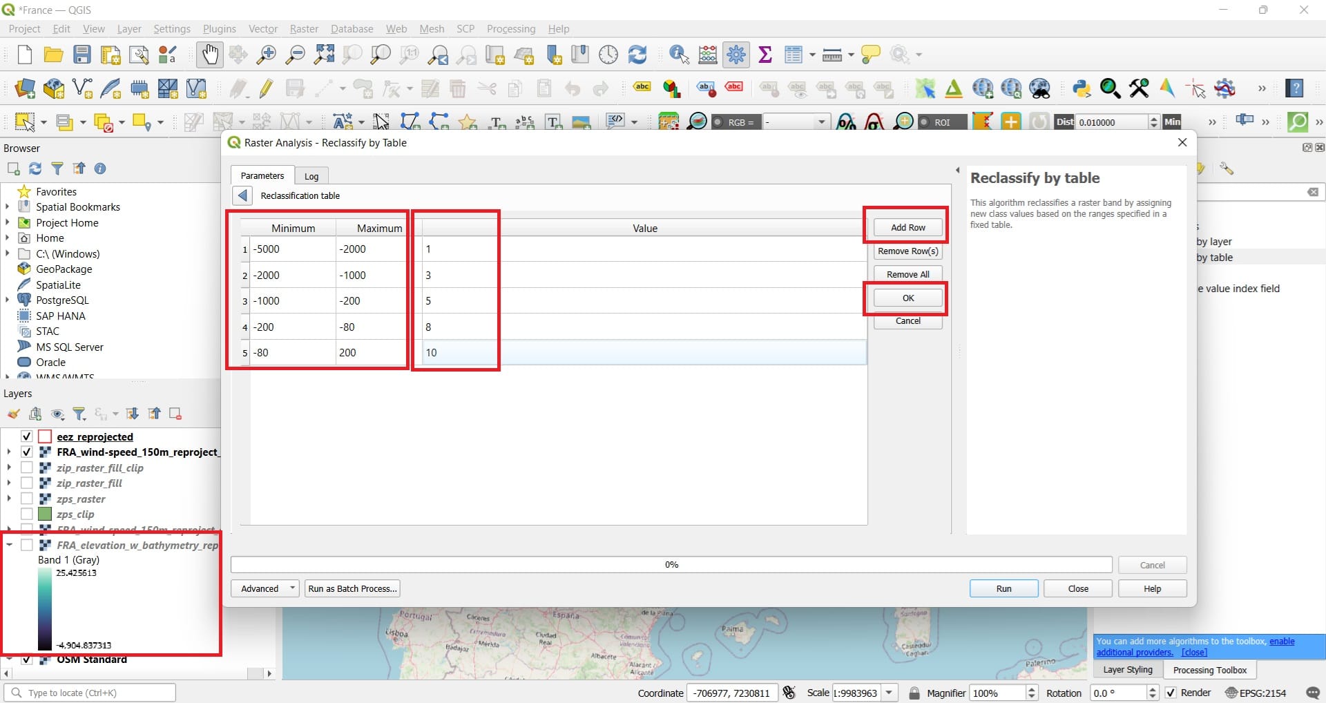
Let’s try a new tool to process our wind and bathymetry data! It’s the ‘Reclassify’ tool if we search on the ‘Processing Toolbox’ (see the image below). The ‘Reclassify by Table’ tool change the pixel values of our raster files based on a categorization we provide! 

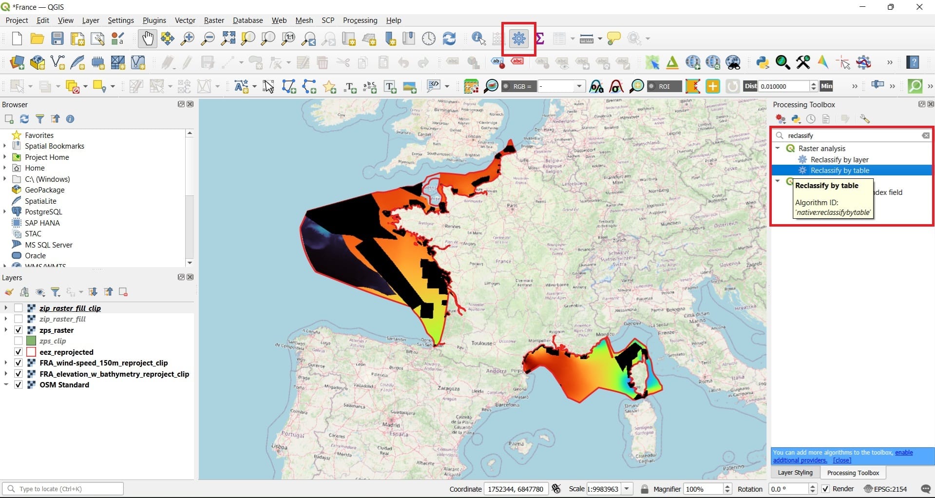
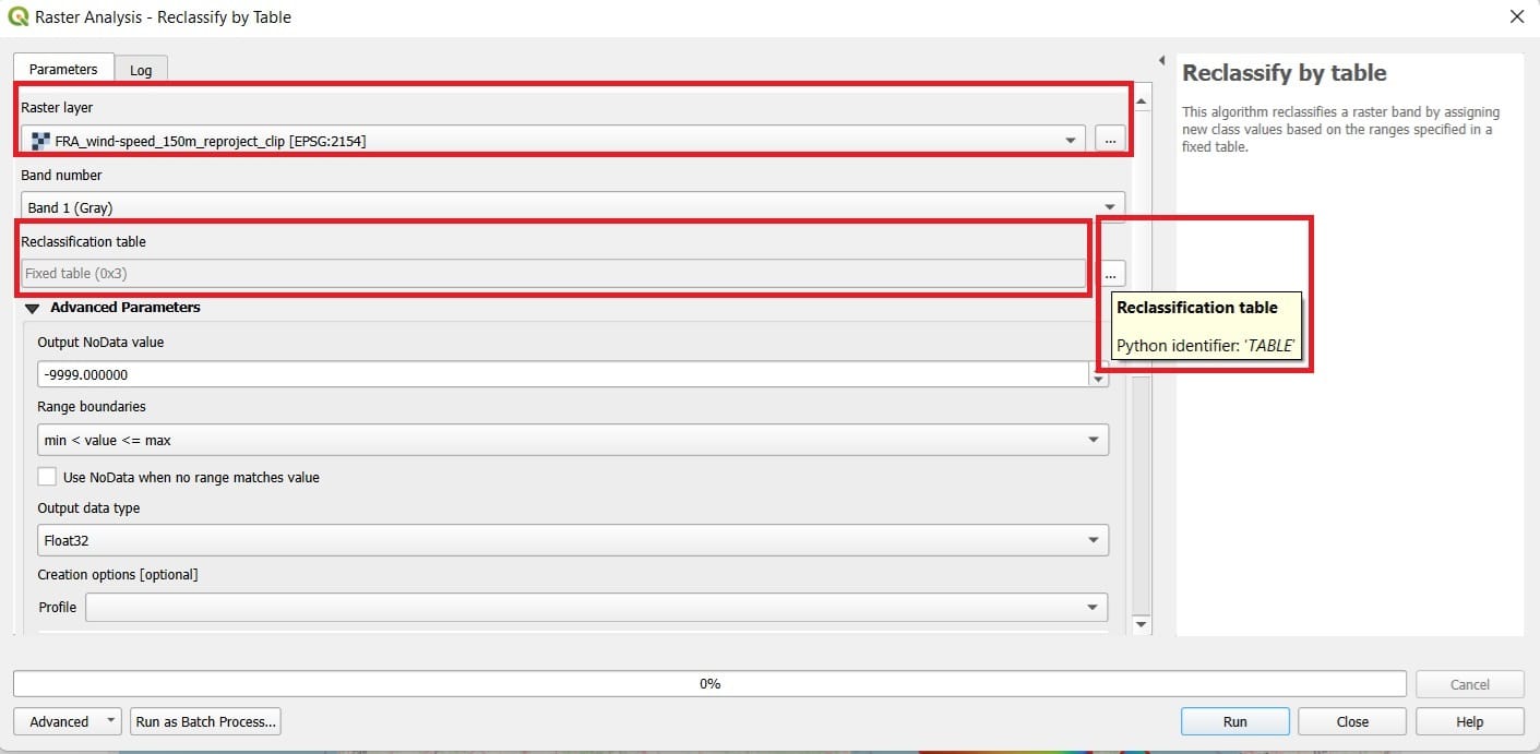
In the ‘Reclassify by Table’ tool we select:

• Raster layer: FRA_wind-speed_150_reproject_clip
• Reclassification table: Select the three dots icon to create a new table

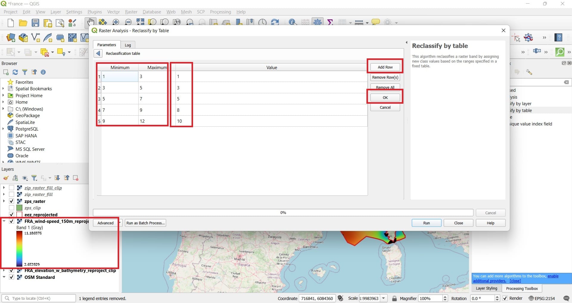
In the new window with the Reclassification table we select:

• Add row: 5 times for 5 rows since we’ll have 5 new classes
• Minimum Maximum: We set the wind speed values per class. For example, wind speed category no.1 has values between 1-3 m/s. How can we see that? By checking the min-max values of the wind speed raster layer in the ‘Layers’ window or by double-clicking on the raster layer > Information > Min-Max values. The min value is 2.6 and the max 11.18.
• In the Value tab: We set the scores we want, for example, the new scores per wind class we want to assign. For example, we consider a low value of 1 for the wind speed class 1-3, a value of 10 for wind speeds between 9-12 etc. (we increase the maximum value to 12, in order to be sure that all values are included!)
• We press OK.
• We scroll down and we Save as layer our new file with the name ‘FRA_wind-speed_150_reproject_clip_reclass’
• Press ‘Run’

Here is the result! Now we can see that the wind speed values have been transformed to score values (good or bad, depending on the color).

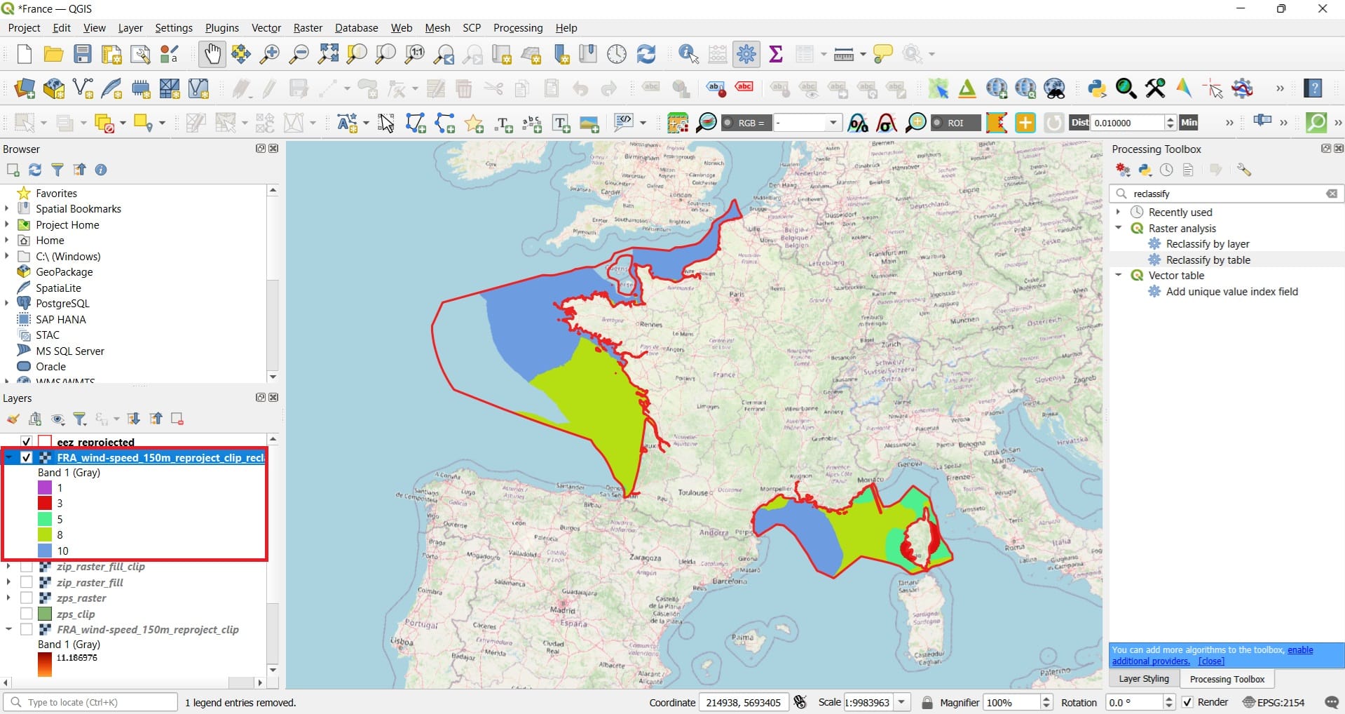
If you want to see similar colors, you just double-click on the new raster layer > ‘Symbology’ > ‘Palletted/Uniques Values’ > ‘Classify’

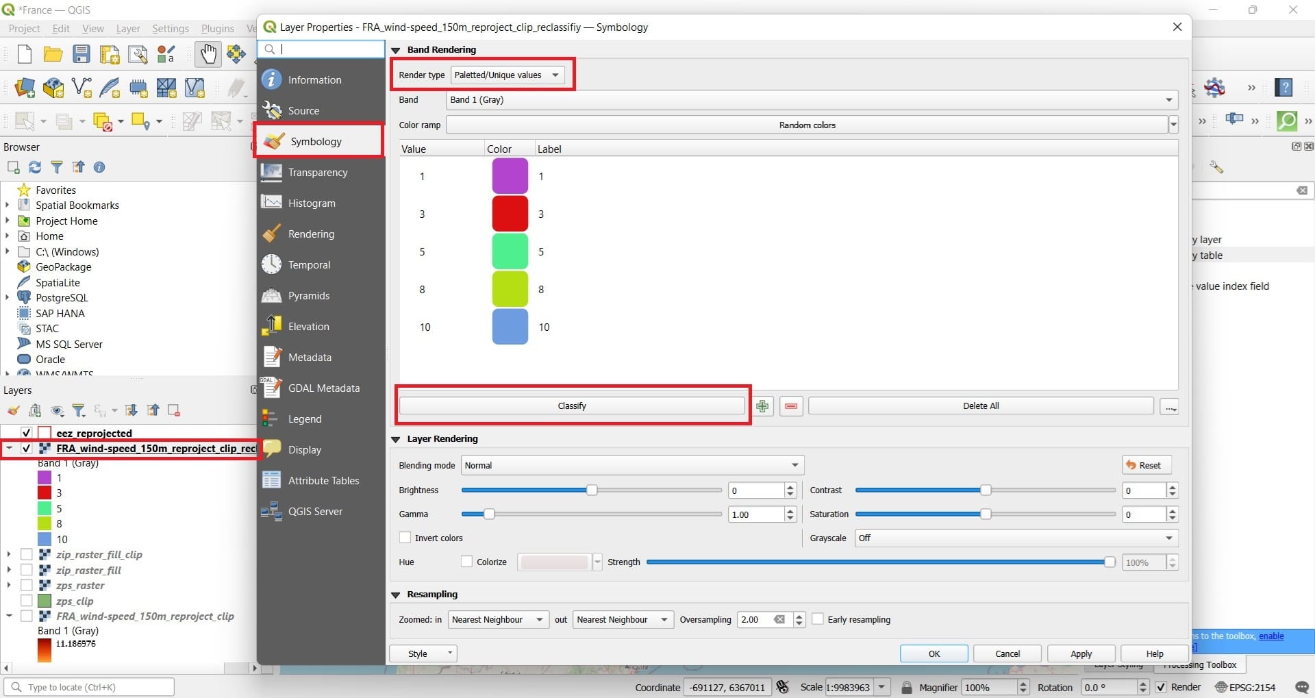
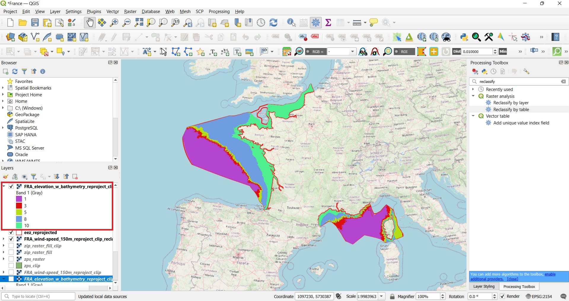
We follow the same process for the bathymetry raster:

• Add row: 5 times for 5 rows since we’ll have 5 new classes
• Minimum Maximum: We set the bathymetry values per class. For example, bathymetry category no.1 has values between -5000-(-2000) meters depth. We see that by checking the min-max values of the bathymetry raster layer in the ‘Layers’ window or by double-clicking on the raster layer > Information > Min-Max values. The min value is -4904 and the max 25.
• In the Value tab: We set the scores we want, for example, the new scores per wind class we want to assign. For example, we consider a low value of 1 for depths between -5000-(-2000) meters, a value of 10 for depths -80 – 200 etc. (we increase the maximum value to 200, in order to be sure that all values are included!)
• We press OK.
• We scroll down and we Save as layer our new file with the name ‘FRA_elevation_w_bathymetry_reproject_clip_reclassify’
• Press ‘Run’

The result will look like the image below, if we change the Symbology like we did in the previous step! Now we can see that the bathymetry values have been transformed to score values (good or bad, depending on the color).

But, why did we apply all these complex functions? Let’s find out in the next lesson!

You may also take a look on the following videos, explaining how to clip and reclassify rasters…

✅ Wrapping Up

You’ve now completed the lesson on Basic Raster Processing in QGIS, where you practiced key skills such as clipping raster layers, filling NoData gaps, and converting vector features into raster format. These steps may seem technical—but they’re far from pointless!

Each of these processes is a building block for more advanced spatial analysis. In fact, the work you’ve done has prepared you to take a major step forward: in the next lesson, we’ll use these exact tools and workflows to conduct our first in-depth multi-criteria analysis for a real-world Offshore Wind Energy project.

So well done—and get ready to turn processed data into informed, spatially grounded decisions! ⚡🌊📊

Useful links

1. Global Wind Atlas: Downloading raster wind and bathymetry data
2. MarineRegions: Downloading Exclusive Economic Zone data
3. INPN: Données du programme Natura 2000 (only for France)