Coordinate Reference Systems (CRS)
Introduction to Coordinate Reference Systems (CRS)
In GIS, all spatial data—whether downloaded, created, processed, or exported—must be accurately tied to a location on the Earth’s surface. This is made possible through Coordinate Reference Systems (CRS), which define how geographic data is mapped onto a flat surface. Understanding CRS is essential for ensuring that your data aligns correctly, especially when working with multiple datasets from different sources.
In this lesson, you will explore how different Coordinate Reference Systems (CRS) work and the differences between Geographic and Projected Coordinate Reference Systems (CRS).
By the end of this lesson, you will:
✅ Understand the difference between geographic and projected coordinate systems.
✅ Avoid common issues related to CRS mismatches in your spatial analysis.
As explained in the QGIS training course “A Gentle Introduction to GIS – Coordinate Reference Systems” [1], map projections are methods used to represent the curved surface of the Earth on a flat surface—like a paper map or a computer screen. In simple terms, a map projection transforms the Earth’s 3D spherical shape into a 2D flat map. There are two main types of coordinate systems: geographic coordinate systems, which use latitude and longitude to describe positions on a spherical surface, and projected coordinate systems, which represent the curved surface of the Earth on a flat map using linear units like meters.
Let’s begin by understanding how CRS ensures your data always knows where it belongs!
Representing the Earth’s surface
Data is typically made up of numerical values. Spatial data like we saw in the previous lesson is no different, but it also contains location information that allows it to be accurately positioned on the Earth’s surface. This location data is based on a coordinate system, which serves as a reference framework. It enables users to locate features geographically, align datasets with one another, perform accurate spatial analysis, edit and update data, and produce meaningful maps.
All types of spatial data, whether vector (points, lines, polygons), rasters, or labels, are created within a coordinate system. Coordinates can be expressed in a variety of units such as decimal degrees, meters, kilometers, or feet, depending on the context. Selecting the appropriate unit of measurement is a crucial first step in defining a coordinate system that will correctly position your data in GIS platforms, ensuring that it aligns properly with other layers in your project [2].
Thus, a Coordinate Reference System (CRS) defines how that two-dimensional map relates to real-world locations. Choosing the right projection and CRS depends on several factors, including the geographic area you’re working in, the type of analysis you’re conducting, and the available data sources. Making the right choice ensures spatial accuracy and prevents distortions in your and your students GIS project.
A traditional method of representing the earth’s shape is the use of globes. Over time, the shape of the Earyh surface has been geometrically represented as a plane, a sphere, a spheroid, and an ellipsoid. For many years, humans have attempted to measure the parameters that would allow for a mathematical description of the Earth’s shape initially, and later, of other unknown quantities. This effort aimed—and still aims—at determining an optimal shape that most accurately represents the Earth’s surface!
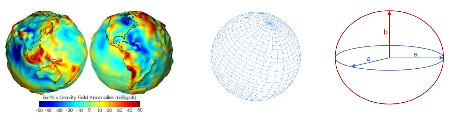
The image above illustrates different representations including the surface of the Geoid (left), the sphere as a reference surface of the Earth, with meridians and parallels (middle) and the rotational ellipsoid (ellipsoid of revolution) (right) [3]. Although globes preserve the majority of the earth’s shape and illustrate the spatial configuration of continent-sized features, they are very difficult to carry in one’s pocket. They are also only convenient to use at extremely small scales (e.g. 1:100 million, map scale refers to the factor of reduction of the world so it fits on a map) [4].
In Geographic Information Systems (GIS), thematic maps often rely on large-scale datasets—typically at scales of 1:250,000, 1:50,000 or larger—to provide detailed spatial information. Attempting to represent such detail on a globe would be impractical due to the size and cost of production, as well as the difficulty in handling and transporting such a model. To address this, cartographers have developed map projections, which are mathematical techniques that transform the Earth’s three-dimensional, spherical surface into a two-dimensional representation on flat media, such as paper maps or digital screens. This transformation is essential for accurately displaying spatial data in a manageable format [4, 5].
Consequenlty, map projections are essential tools in cartography, enabling the representation of the Earth’s three-dimensional surface on two-dimensional media like paper maps or digital screens. To conceptualize how map projections work, imagine placing a light source inside a transparent globe with opaque features representing Earth’s geography. By projecting these features onto a surrounding surface—be it a cylinder, cone, or plane—and then unrolling that surface, we obtain a flat map. This process gives rise to three primary families of map projections, each defined by the geometric surface onto which the globe is projected: cylindrical, conic, and planar (also known as azimuthal) projections [4, 6, 7].
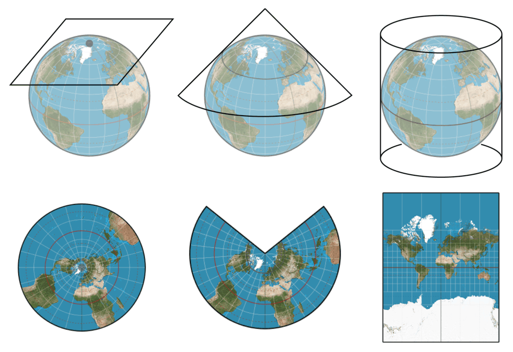
As Battersby (2017) highlights, with respect to projections, the above-illustrated surfaces can be used to ‘wrap’ a reference globe, and, with an imaginary light shining on the reference globe, the shadows of the features of the globe are transferred onto the developable surface. In particular:
Cylindrical Projections: In cylindrical projections, the globe is projected onto a cylinder that envelops the Earth. When unrolled, this cylinder produces a rectangular map where meridians and parallels intersect at right angles. A well-known example is the Mercator projection, which preserves angles, making it useful for navigation, but distorts area, especially near the poles.
Conic Projections: Conic projections involve projecting the globe onto a cone placed over the Earth, typically touching it along one or two lines of latitude known as standard parallels. When the cone is unrolled, it yields a map where meridians radiate from a central point and parallels appear as arcs. This projection is particularly useful for mapping mid-latitude regions with an east-west orientation, such as the contiguous United States.
Planar (Azimuthal) Projections: Planar or azimuthal projections project the globe onto a flat plane that touches the Earth at a single point, often the poles. This results in a circular map where distances and directions from the central point are preserved. Such projections are ideal for polar regions and are commonly used in air route maps. Each of these projection families offers unique advantages and is chosen based on the specific requirements of the map’s purpose, the region being represented, and the importance of preserving certain spatial properties like area, shape, distance, or direction. Understanding these families aids cartographers and GIS professionals in selecting the most appropriate projection for their mapping needs.
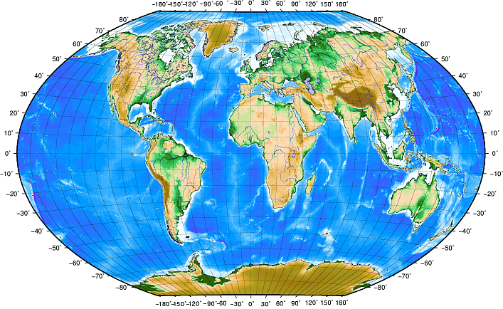
Accuracy of map projections: Map projections are never absolutely accurate representations of the spherical earth. As a result of the map projection process, every map shows distortions of angular conformity, distance and area. A map projection may combine several of these characteristics, or may be a compromise that distorts all the properties of area, distance and angular conformity, within some acceptable limit. Examples of compromise projections are the Winkel Tripel projection and the Robinson projection, which are often used for producing and visualizing world maps [4].
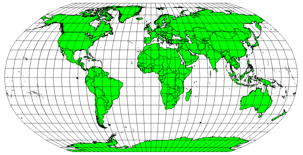
The Robinson projection (see image above) is a compromise where distortions of area, angular conformity and distance are acceptable [4].
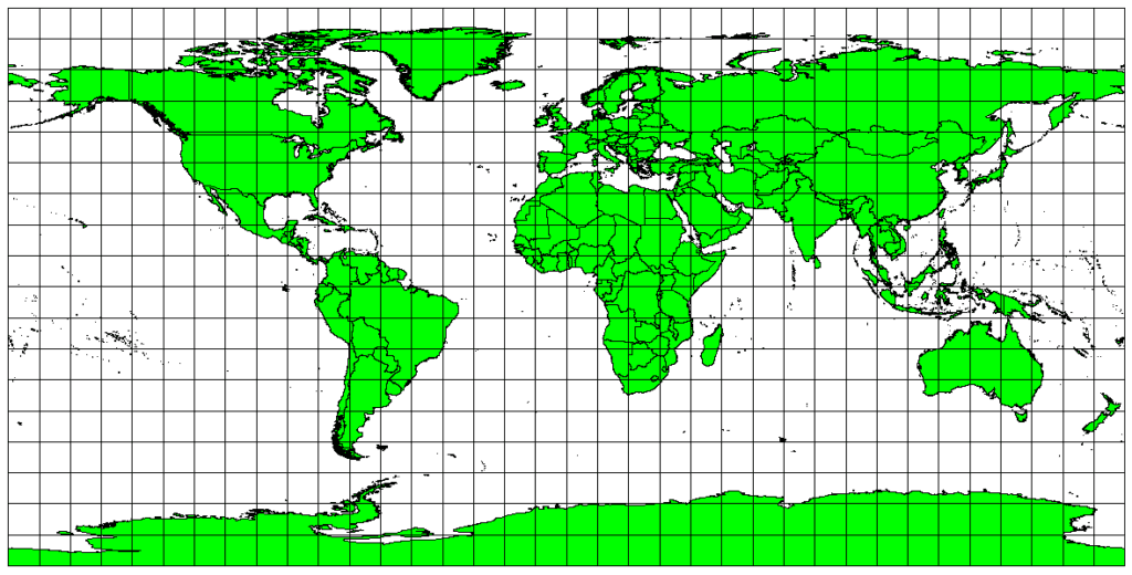
The Plate Carree Equidistant Cylindrical projection, for example, is used when accurate distance measurement is important [3].
Apart from the above-mentioned projections, there are also the so called ‘Map projections with angular conformity’ [4]. When working with a globe, the main directions of the compass rose (North, East, South and West) will always occur at 90 degrees to one another. In other words, East will always occur at a 90 degree angle to North. Maintaining correct angular properties can be preserved on a map projection as well. A map projection that retains this property of angular conformity is called a conformal or orthomorphic projection. These projections are used when the preservation of angular relationships is important. They are commonly used for navigational or meteorological tasks. It is important to remember that maintaining true angles on a map is difficult for large areas and should be attempted only for small portions of the earth. The conformal type of projection results in distortions of areas, meaning that if area measurements are made on the map, they will be incorrect. The larger the area the less accurate the area measurements will be. Examples are the Mercator projection or the Lambert Conformal Conic projection.
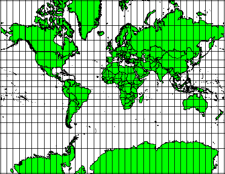
The Mercator projections used where angular relationships are important, but the relationship of areas are distorted.
The Mercator projection is a cylindrical map projection presented by the Flemish geographer and cartographer, Gerardus Mercator, in 1569. This map projection is practical for nautical applications due to its ability to represent lines of constant course, known as rhumb lines, as straight segments that conserve the angles with the meridians. Although the linear scale is equal in all directions around any point, thus preserving the angles and the shapes of small objects, the Mercator projection distorts the size of objects as the latitude increases from the equator to the poles, where the scale becomes infinite (see gif visualization below). A classic example of the distortion that this projection causes is that Greenland, Russia and Antarctica appear much larger than they actually are (red polygons on the image below) relative to land masses near the equator, such as Central Africa. Another distortion this projection causes is that Greenland appears larger than Australia, while in actuality Australia is approximately three and a half times larger than Greenland [8].
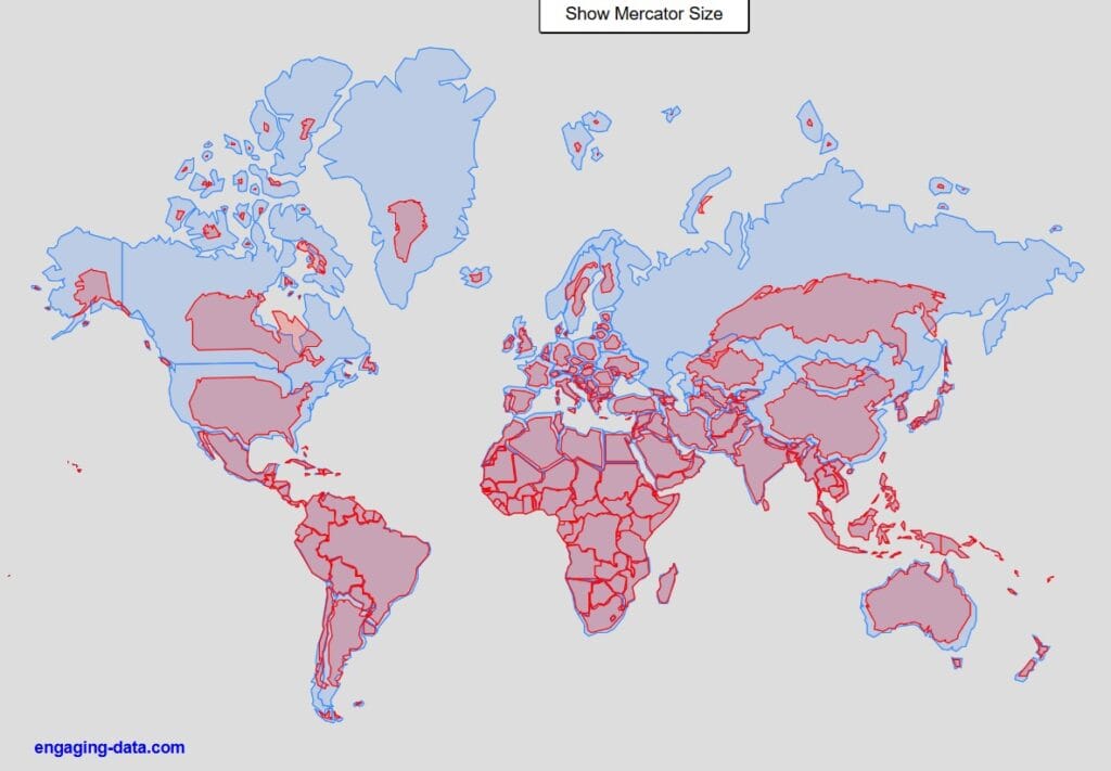
See the engaging-data app here. You may also use the TrueSize Game showing how the Mercator projection distorts the size of objects as the latitude increases from the equator to the poles!
Coordinate Reference System (CRS)
With the help of coordinate reference systems (CRS) every place on the earth can be specified by a set of three numbers, called coordinates. In general CRS can be divided into geographic coordinate reference systems and projected coordinate reference systems (also called Cartesian or rectangular coordinate reference systems).
🌍 Geographic Coordinate Systems (GCS)
A Geographic Coordinate System (GCS) is a framework that enables the precise identification of locations on Earth’s surface using a set of numerical values. These values are typically expressed in degrees of latitude and longitude, and sometimes include an elevation component.
🧭 Latitude and Longitude
- Latitude: Measures the distance north or south of the Equator (0° latitude). It ranges from 0° at the Equator to 90° at the poles. Positive values indicate locations in the Northern Hemisphere, while negative values denote the Southern Hemisphere.
- Longitude: Measures the distance east or west of the Prime Meridian (0° longitude), which passes through Greenwich, England. It spans from 0° to 180°, with positive values to the east and negative values to the west.
These coordinates form a grid system that allows for the pinpointing of any location on Earth (see image below).
🌐 World Geodetic System 1984 (WGS 84)
The World Geodetic System 1984 (WGS 84) is the standard GCS used globally, particularly in GPS technology and various mapping applications. It defines an Earth-centered, Earth-fixed coordinate system and a geodetic datum, providing a consistent frame of reference for geospatial data.
WGS 84 utilizes an ellipsoidal model of the Earth, accounting for its slightly flattened shape at the poles and bulging at the equator. This model enhances the accuracy of location data across different regions.
📏 Consistency in Measurement
An important characteristic of latitude lines is their consistent spacing. Each degree of latitude is approximately 111 kilometers (or 60 nautical miles) apart, regardless of the location on Earth. This uniformity aids in the accurate calculation of distances between points.
🗺️ Projected Coordinate Systems (PCS)
A Projected Coordinate System (PCS) is a spatial reference framework that represents the Earth’s curved surface on a flat, two-dimensional plane. This transformation is achieved through mathematical techniques known as map projections, which convert geographic coordinates (latitude and longitude) into planar coordinates (X and Y).
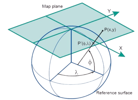
Example of a map projection where the reference surface with geographic coordinates (f,l) is projected onto the 2D mapping plane with 2D Cartesian coordinates (x, y) [image source: KartoWeb].
📐 Understanding the Components of PCS
A typical PCS comprises the following elements:
- Map Projection: The mathematical method used to translate the Earth’s three-dimensional surface onto a two-dimensional plane.
- Geodetic Datum: A model that defines the size and shape of the Earth, serving as a reference point for the coordinate system.
- Coordinate System: Defines the X (horizontal) and Y (vertical) axes on the flat map, allowing for precise location referencing.
- Unit of Measure: Specifies the measurement units (e.g., meters or feet) used for the coordinates.
These components work together to provide an accurate and consistent method for mapping and spatial analysis.
🌐 Commonly Used Projected Coordinate Systems
One widely adopted PCS is the Universal Transverse Mercator (UTM) system. UTM divides the world into 60 zones, each 6 degrees of longitude wide, providing a high level of accuracy for regional mapping. Below is a list of commonly used projected Coordinate Reference Systems (CRS) along with their EPSG codes for Greece, Cyprus, Portugal, Austria, Bulgaria, and Sweden (retrieved from EPSG.io: Coordinate Systems Worldwide). Why do we need the EPSG codes? Because it’s way more easier to search for those coordinate systems in GIS platforms like QGIS!
Greece (GR)
- CRS Name: GGRS87 / Greek Grid
- EPSG Code: 2100
- Description: This system is based on the Greek Geodetic Reference System 1987 and is widely used for engineering surveys and topographic mapping within Greece.
Cyprus (CY)
- CRS Name: CGRS93 / Cyprus Local Transverse Mercator
- EPSG Code: 6312
- Description: Adopted by the Cyprus Department of Lands and Surveys, this CRS utilizes the WGS 84 ellipsoid and is employed for cadastre, engineering surveys, and topographic mapping.
Portugal (PT)
- CRS Name: ETRS89 / Portugal TM06
- EPSG Code: 3763
- Description: This system is the official CRS for mainland Portugal, based on the ETRS89 datum, and is used for medium-scale topographic mapping.
Austria (AT)
- CRS Name: MGI / Austria GK M31
- EPSG Code: 31285
- Description: Utilizing the MGI datum and Bessel 1841 ellipsoid, this CRS is applied in engineering surveys and topographic mapping across Austria.
Bulgaria (BG)
- CRS Name: BGS2005 / CCS2005
- EPSG Code: 7801
- Description: Based on the Bulgarian Geodetic System 2005, this CRS is used for cadastre, engineering surveys, and topographic mapping throughout Bulgaria.
France (FR)
- CRS Name: RGF93 / Lambert-93
- EPSG Code: 2154
- Description: This system is based on the Réseau Géodésique Français 1993 (RGF93), aligned with the European Terrestrial Reference System 1989 (ETRS89). It is the official coordinate reference system for cartographic and geospatial applications across metropolitan France, commonly used in mapping, cadastral, and engineering projects.
Sweden (SE)
- CRS Name: SWEREF99 TM
- EPSG Code: 3006
- Description: Adopted in 2003, this CRS replaces the older RT90 system and is used for various mapping and surveying applications across Sweden.
These coordinate systems are essential for accurate mapping, surveying, and geospatial analyses within their respective countries. Each system is tailored to the specific geodetic and cartographic needs of the region it serves.
⚖️ Advantages of Using PCS
- Accurate Distance and Area Measurements: PCS allows for precise calculations of distances and areas, which is essential for engineering, construction, and land management.
- Consistency Across Maps: By using a standardized coordinate system, different maps can be overlaid and compared accurately.
- Facilitates Spatial Analysis: PCS enables complex spatial analyses, such as distance measurementm network routing and terrain modeling, by providing a uniform framework.
Understanding Projected Coordinate Systems is crucial for professionals engaged in geospatial fields, as it underpins accurate mapping, analysis, and decision-making processes. We will explore all these capabilities during our next course on Spatial Analysis & Data Processing!
Useful links
- QGIS: Coordinate Reference Systems
- ESRI: Coordinate systems, map projections, and transformations
- NTUA (Cartography Laboratory): Geographic Information Science (GIS) – In Greek
- ESRI: Choose the right projection
- ESRI: Projection types
- UCGIS: Geographic Information Science & Technology Body of Knowledge Visualization and Search
- Fletcher S.J. (2023). Numerical Modeling on the Sphere. Data Assimilation for the Geosciences (Second edition), From Theory to Application
pp. 485-555 - QGIS: Working with projections
1 Comment
Submit a Comment
You must be logged in to post a comment.
It would be nice if you gave us videos on the mathematical concepts and calculations of each projection